Abstract
This study was conducted to develop a 2D model from the 1D model. 1D models, which have been used for flood modeling have shown significant weaknesses, which prompted research into 2D modeling of floods. The main weaknesses of the 1D model are that they are unsuitable for urban and intricate systems modeling, leading to the creation of the 2D model. This study was conducted using artificial modeling, which was based on an abstract representation of real-world flood events in the Taco River and the flow of water in real urban areas. The modeling was done using the PCSWMM software with the objectives of developing the 2D model from the 1D model.
The results show that the 2D model was created by use of interconnected nodes and cells and links which represent the physical features of the area being modeled. There is an excellent agreement between the 1D and 2D models based on the modeling results using the PCSWMM software, which is a new but effective tool for modeling. The PCSWMM tool was evaluated for use in practical situations and coherent results were established, showing that the minimum requirements were achieved to model the flow of floodwater in complex urban areas with several nodes and interconnected cells.
Introduction
According to Awbi (1989), flooding is one of the major emerging concerns around the globe. In recent years most of the natural disasters around the world have been the result of major floods, which have affected over half of the world’s population (UNISDR, 2014). The rapid trend towards urbanization and climate change are the key factors of the increase in the frequency of floods. According to Chen, Djordjevic, Leandro, and Savic (2007), the effects of floods in developed areas are also high as it is directly related to the high number of people living and working in these urban areas. This effect can be reduced by using the solution achieved by modeling and preparing in advance for the predicted effects of the floods.
PCSWMM 2D is a software developed by EPA in 2011 integrating the previous 1D modeling software. These are used for flood modeling and are helping to plan and design the strategies for flood management. This software overcomes the limitation in the 1D model such as flow direction and comes with various new features for better understanding and accuracy.
Project definition
The project is to work on the new 2D hydraulic/hydrological modeling of urban catchments using PCSWMM 2D. As these 2D models are recently been available so 1D will also be used in the initial stage to check the accuracy of 2D models.
The key project’s objective:
- To understand 2D hydraulic flood modeling using PCSWMM for real-time and risk assessment application.
- To evaluate features, capabilities, accuracy, and feasibility of PCSWMM
Project Benefits
Damage as a result of flooding has been a serious issue around the world, with the increase in floods in the last decade it is important to work on risk assessment and real-time flood modeling and management. This study will assist in understanding the risk and destruction caused by flooding. It will help to reduce the effects of pre-assessment of floods and the directions of flow.
Project Deliverable
The understanding from the experiment would be the deliverable of this project which is expected to contribute to real-life flood management and reduce the effect of floods around the globe in real-time.
Literature review
Research rationale and significance of the study
The rationale of the study is to determine how the 2D model, which is developed from the 1D model, can be used to provide better, modeling results where the 1D model cannot be used to overcome the limitations of the 1D model (Vojinovic & Tutulic 2009). The significance is to enable accurate modeling to be done for urban areas and other areas, which cannot be modeled using 1D modeling (Chen, Djordjevic, Leandro & Savic 2007).
1D modeling
Studies of the use of one-dimensional models using different flood simulations floods based on Barré de Saint Venant’s equations, which are defined by floodwater moving in specific directions have revealed several weaknesses (Zaghoul & Al-Shurbaj 1990). When carrying out simulations, the assumption that floodwater takes a unidirectional flow according to the shape of the channel along which the water flows is erroneous because such a situation does not occur in practice. Translating the results of the flow of water under the predictions of the Saint-Venant equations and the risks posed are flawed because the flow of water along the flood plains is not uniform (Vojinovic & Tutulic 2009). In addition, the flow patterns cannot be modeled effectively using one-dimensional modeling because of the presence of roads and buildings, and other infrastructure.
According to Vojinovic and Tutulic (2009), when floodwater simulations show unpredictable flow patterns, which are not properly defined using 1D modeling in urban areas using channels with different shapes and sizes, it makes 1D modeling difficult and the results inapplicable over a wide range of situations (Schmitt, Thomas & Ettrich 2004). The results make it difficult to model the flow of water in a flood situation in urban areas using 1D modeling techniques.
1D and 2D modeling
A distinction between 1D modeling and 2D modeling shows that when doing 1D modeling, the main assumptions are that the flow of water is treated as flowing in a longitudinal direction in a flood plain or water channels (Rungo & Olesen 2003). In addition, the law of conservation of mass and energy is used in the derivation of the equations of 1D modeling. On the other hand, 2D modeling is done by integrating the equations of the flow of water over the depth of flow of water to determine the average velocities of the flowing water at different depths based on the finite element methods and other appropriate numerical methods (Sanders 2007).
To create a 2D model from the 1D model, it is important to understand how the 1D model is created using different flow patterns of floodwater using steady and unsteady flow calculations (Rungo & Olesen 2003). Typically, when modeling the flow of water on a 1D model, the assumptions are that the cross-sectional velocity of the flow of water is uniform, water does not experience vertical accelerations, and the streamline curvature is small, which makes the pressure exerted by the water on the surface to be hydrostatic. Martin, LeBoeuf, Dobbins, Daniel, and Abkowitz (2005) argue that it is possible to account for the turbulence and boundary friction using laws of resistance, which are similar to the laws used to determine the steady flow of water on even surfaces. The equations shown below have been derived using the law of conservation of momentum.
The above equation is defined by different variables, which include t the time, x the channel distance, T (h. t), R the lateral flow, T the free surface area, A the wetted area, and Sr and So, the slop, which is the friction, and g the gravitational pull of the earth (Kuiry, Sen & Bates, P D 2010). The slope of the bed and the friction of the slope are respectively given by:
The manning friction is n in the equation and the wetted perimeter is given by p(x, h). Assuming that the flow occurs in a rectangular channel with A as the cross-sectional area, and by factoring other variables, the resulting equation becomes:
In comparison, the equation for the manning friction for the 2D model becomes:
The manning friction for the 1D model becomes:
The weaknesses of the 1D model when compared with the 2D model provide the rationale for 2D modeling using capabilities of the PCSWMM software (Kuiry, Sen & Bates 2010).
2D Modeling
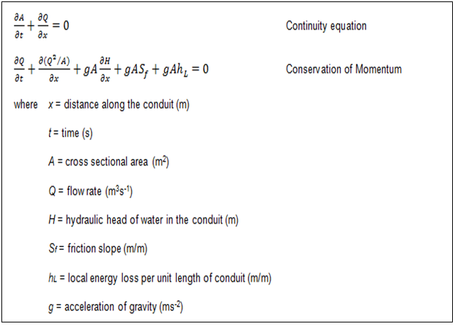
It is important to note that the 2D models are based on hyperbolic partial differentiation, which is based on equations derived from shallow water integration. The assumption used to derive the 2D numerical models includes the similarities between the depth of the water and the surface curvature distributions (Mark, Weesakul, Apirumanekul, Aroonnet & Djordjević 2004). The finite differential method of the software in use can be used to derive the equations used to govern the derivation of the model, which are based on the law of conservation of momentum as shown below.
The computational circle is shown below.
The 2D modeling was done in the coastal areas of the flow of floodwater under different situations using different variables. However, the 2D modeling was done by considering the second equation of the conservation of momentum.
However, it is important to determine a correct solution under extreme flow circumstances (Mark, Weesakul, Apirumanekul, Aroonnet & Djordjević 2004). It has been established that flooding can be modeled using the PCSWMM with a greater degree of accuracy compared with the use of other numerical methods. PCSWMM relies on the powerful GIS engine to model the 2D flow of floodwater in the rural and urban areas, the flow routing of rainwater, and the dynamic flow of water under different conditions and variables. In addition, the software enables modeling to be done without any restrictions because it can account for modeling differences of hydrological processes including rainwater, groundwater, and surface water (Horritt & Bates 2002).
Typically, 2D modeling using the PCSWMM software is an extension of 1D modeling using PCSWMM. Each component of the computational cells used in 1D modeling, which lead to the 2D modeling are derived using numerical methods and can be formulated using the St-Venant equations are determined using the PCSWMM software. The reason is that different cells of the 1D model are integrated into the PCSWMM software and can be used to create 2D modeling cells to enable the creation of an accurate 2D model (Greenberg & Leroux 1996).
It is has been established that “homogeneous fluids are solved along with each component of a computational cell, over a network of junctions and open conduits that represents the problem hydrography, bathymetry or topography’ (Greenberg & Leroux 1996). PCSWMM 2D “does not consider Coriolis force (which is a factor for very large study areas), wind shear forces or turbulent eddy viscosity” (Greenberg & Leroux 1996) based on the continuity and preservation of momentum equations as shown below.
In the above study, a finite approach is used to determine the actual solution to the problem based on approximations, which are used for 2D modeling (Greenberg & Leroux 1996). When considering dynamic situations, 2D nodes are used to provide the framework for conducting the study on a surface area of 0.1 m2. The surface area under consideration consists of interconnected nodes used to preserve continuity (Greenberg & Leroux 1996). The area and nodes under consideration have different lengths and sizes and the floodwater being modeled has different magnitudes of velocities. It is possible to use the software to calculate the average floodwater velocity, which is the sum of the velocities of the floodwater flowing away from the cells.
It has been established that 2D models have been widely used in flood risk evaluations because the models can provide high-resolution digital elevations combined with the increase in computing power and resources (Ferguson & Suckling 1990). The software has been used to evaluate other techniques based on 2D models, which are used to create different models (Ferguson & Suckling 1990). It has further been established that the model provides an effective source of data about floods and the behavior of flood waves, velocities, and fluxes for the computational domain used in the study.
On the other hand, it has been established that 2D models require high computational capabilities and resources to model. However, when compared with other models, the model requires fewer storage cells to model the behavior of particles, making the results obtained from 2D models more accurate than results obtained from the 1D model (Chen, Hsu, Huang & Lien 2011).
Modeling limitations
When carrying out the 2D modeling, several problems are encountered because the solutions obtained are based on the St-Venant 1D model equations. To address the limitations, it is important to ensure that the flow cells used in the study are 1 dimensional. The study makes assumptions that the windy force and eddy currents which arise because of the flow of water are insignificant, and the depth or width of the water is significantly smaller than the wavelength of the flow model (Chen, Hsu, Huang & Lien 2011).
To ensure that the results are accurate and reliable, it is important to use a depth ratio of 5 to the cell resolution to minimize the effects of boundary friction. The model run time can be minimized by integrating both 1D and 2D models to determine the solutions. In addition, a mesh solution can be used because it reflects the conditions of the flood water environment. Some of the examples used in the study include the PCSWMM Sediment Buildup and wash-off events to ensure that the results were consistent with the requirements of running the 2D model tests.
Features, capabilities, accuracy, and feasibility of PCSWMM
Different programs have been used to evaluate 1D and 2D models of the flow of floodwater using different topographical features. Studies conducted at Massachusetts using PCSWMM software based on default parameters to represent the flood flow conditions revealed data, which shows the level of accuracy and effectiveness of the software. Some of the parameters were “Manning’s equation, maximum and minimum infiltration rates and wash-off methods model” (Chen, Hsu, Huang & Lien 2011), which were related to the 1D and 2D models.
The parametric assumptions used in the study include ‘evapotranspiration’, which describes the rate of loss of water into the atmosphere, pan-evaporation, depression storage, and Manning’s equation, which were derived empirically using open channels of flowing flood water. Based on Manning’s equation, it was clear that the results of the modeling process were influenced by shallow, sheet, and continuous characteristics of the flow of the floodwater model (Chen, Hsu, Huang & Lien 2011). The results were subjected to sensitivity analysis using the parameters tabulated in the table below.
Specific parameters, which were evaluated in the study, include surface width, depression storage, and the rate of evaporation of the flood water by using several runs of the program to conduct sensitivity analysis using different parameters. The results were obtained from an experimental study done on a 5 acre of land, which provided sufficient space to alter the parameters and make observations about the cumulative effects of the runoff water model (Chen, Hsu, Huang & Lien 2011).
After running the program several times, the results showed that certain parameters, which include unit sizing were not affected, showing that the model was insensitive to the changes of the parameters. On the other hand, when changes were made on the parameters, no discernible changes in the behavior of the model being tested were observed. However, the drainage area had a strong effect on the characteristics of the runoff flood water and the flow rate of the water, which shows that the bigger the area the greater the speed of runoff water when simulated using the software model (Chen, Hsu, Huang & Lien 2011).
Another study to determine the effects of particle size on the use of PCSWMM software showed that the software does not provide instructions on the particle sizes that can be used for simulation input. In addition, a study was conducted to determine the accuracy and performance of the software for determining PCSWMM simulations on rainwater and it was established that PCSWMM was limited in providing accurate data on the performance of rainfall (Rungo & Olesen 2003).
Typically, the program is designed to collect long-term data set from a specific station. The program provides features, which enable the user to adjust a shorter period of rain, which, however, is not recommended to be used in that manner. The output data from the PCSWMM software can be evaluated t determine the accuracy of the software based on the input file data (Rungo & Olesen 2003).
Another study was conducted to determine the effects of the size of the particles used on PCSWMM simulation results. Six installations were used to determine the answer to the question and the input data was obtained from the use of PSD data and other input parameters for other installations were kept constant. The results showed that further studies were necessary to determine the effects of the size of particles on the outcomes of the PCSWMM simulations.
It has been determined that PCSWMM software has a significant number of tools, which can be used in the presentation of results. For instance, studies done to investigate and compare the accuracy PCSWMM software with the Proprietary BMP: Stormceptor STC based on data from 8 impervious areas with a 77% TSS removal using “Stormceptor sizing for TSS removal in the STEP Technology Assessment” recommended that an area of 4 acres was sufficient to achieve different stormwater management simulation strategies (Rungo & Olesen 2003).
For the comparative study to be done an impervious site of 1 acre was used to run two simulations and it was determined from the study that PCSWMM was not sensitive to the rainfall variations. The PCSWMM provides a wide range of capabilities including2Dsimulations including stormwater movement. However, it was determined from the trial runs that the PCSWMM has several limitations when used on 2D models. Those limitations include small variations on the variations shown on 2D model simulations because the 2D model required significant changes in the elevation of the topography of the area being stimulated. In addition to that, when the elevations are too small, the values used can be too small to cause any changes in the simulations.
SWMM5 Components
The SWMM5 components consist of links, nodes, rain gauges, watersheds, time patterns, pollutants, and curves. In addition, the software is defined by “controls, transects, aquifers, unit hydrographs, snowmelt and shapes” (Chen, Hsu, Huang & Lien 2011). The main “components of the program include input file and C code of the simulation engine” (Chen, Hsu, Huang & Lien 201).
Linking 1D with 2D model
A typical example was considered in a study to demonstrate how the 1D model could be linked with the 2D model to create an accurate 2D model (Rungo & Olesen 2003). The study was done on a river where the level of the water could exceed the ground level during a flood as shown on the diagram shown below. The advantage of the 2D model is that it allows the 1D model to be integrated into an existing 2D model by creating a mesh on the 1D model. Typically, the linking can happen in different simulation environments including riverbanks.
A 1d and 2D modeling mesh can be improved when doing the simulations by adding, moving, and deleting the nodes to determine the most appropriate connections between the 1D links with 2D links (Rungo & Olesen 2003). Typically, the inflow can be supplied by the runoff component when the 2D model is connected to the 1D model.
A comparative study shows that the data obtained based on a 1D model integrated into a 2D model led to a 2D profile having multiple nodes joined together. As shown below, the 1D model is linked to the 2D model using the nodes in the diagram.
The points include the extents of the river channels or any other points on the river, which can be modeled using 1D and 2D models (Sanders 2007). By raising the elevation of the identified areas, it is possible to raise the ground level of the floodwater and be consistent with the requirements of modeling using the 2D model. The results of the modeling process lead to the following scenario.
However, three options are available for integrating the 1D model into the2D model and include the 1D model survey consisting of the flood plains, an extension of the 1D model to the between the flood plain and the main river channel, and the walking survey of the river used in modeling as shown below.
The results of linking the 1D model with the 2D model are illustrated below.
Methodology
The study investigated the 2D modeling based on a 1D model to determine the accuracy of the model because it has been recommended to be the best alternative to the 2D model. A 1D model was developed to provide data, which relied on the use of sediment build-up and wash off floodwater resulting from rainwater events. Initial watershed loads were not considered in the study because of the insignificance of the impact of the water loads on the accuracy of the results. In addition, the 2D model validation was done by comparing predicted values with the data yielded from field observations using experimental physical model observations and 2D model predictions. The study used the Toce River in Italy as the source of the physical data because of the high quality based on data obtained from several locations and compared with the use of field data.
The initial water and solid loads before the start of the wash-offs, the investigation considers them to be stochastic variables. The accumulation of solid loads is not a limiting factor in the study. In addition, site-specific data was used to minimize the potential errors of building up the methodology, which was used in the study. In addition, the current research utilized available published reduced-scale data that has been collected through observations based on hypothetical flood plains. To address the problem, the software was downloaded and installed on a computer and the simulation parameters were chosen. The nodes consist of linked rivers and flood plains and the characteristics of the cells that were used in the model were determined using the software to create the flow path and several assumptions were made, which include:
- Lower manning values can be used to model impervious areas
- Higher manning values can be used in areas with poorly maintained lawns.
- The net impact of overland flow discharge, surface width, and runoff volume cannot be precisely determined using numerical methods.
- Additional guidance should be provided when using Horton’s equation for infiltration.
- Literature values provide reasonable confidence that they can be used in 2D modeling reliably.
- 15 minutes were used to analyze the results and data was collected at hourly intervals.
- The density of the water that is used in the model is constant
- The vertical accelerations and curvature of the streamline are negligible making a hydrostatic distribution of pressure possible.
The actual area under which the model was tested is shown below. The geometry, flood areas, the spill geometry of the floodwater, and the building are shown.
The study area is shown below.
The predictions by the 1D and 2D models were done by considering data from the River Clyde in Glasgow City, UK. Typically, the above method uses a nested grid modeling method on 1Dand 2D models because the approach is taught to allow the use of simulations with relatively low resolution. It is possible to identify additional features in the above area when using finer grid resolutions such as flow paths because other bulk characteristics of the flow patterns of the flood water do not have any impact on the resulting model. However, the resolutions can affect the depth, velocities, wavelengths, and patterns of inundation. It has been established that the flow patterns of floodwater can be modeled better using higher resolutions.
Higher resolutions result in higher demands for computational power because of the high number of grids. It is, however, possible to reduce the number of grids because some of them can be accommodated into the model and gradually lead to losses because they may not be used in modeling.
1D and 2D modeling description
The topography of the area used for setting up the physical experiment is 50 m long (Sanders 2007). The area used for the study was reduced to using a scale of 1: 100 to ensure that the specifications are consistent with the program requirements, creating a reach of 5 km with a topographical resolution of 5 m. The PCSWMM program was set and the parameters and other simulation features were selected from the drop-down menus (Sanders 2007).
To set up the simulation, the requirements were defined for selecting the area and the specific point to be modeled using the above software. Any building within the elevation of the flow of the floodwater being modeled using the 1D and 2d models was included in the computerized grid and considered to be obstacles to the flow of the floodwater. However, the floodwater could flow out of any building through the window openings, cracks in the outer walls, and any openings in the buildings. In addition, it is possible to get lower water levels and velocities because of the nodes or cells that interfere with the flow of floodwater (UNISDR, 2014). The origin is located somewhere below the river and acts as the reference point for all other areas.
In the above experiment, two urban district layouts were used consisting of the staggered and aligned buildings. On the other hand, the original topography consists of 20 buildings, which are numbered consecutively as shown below.
The water depths probes are located in the following table as per their coordinates.
On the other hand, the bounding layers in the above setup were defined using the attributes of the 1D and 2D models because water can flow around obstacles. The layers define the attributes of the area being modeled using the software.
Upstream boundary conditions
It is possible to ensure that the boundary condition of the experimental database don the water level can be maintained to ensure that the desired hydrographs of the low, medium and high relative to the highest level can be achieved as shown on the following diagram.
Laboratory runs
After the setups were done, a series of experiments were run to determine the answers to the research objectives and the results are shown below. Typically, when the experiment was run, upstream reflections were avoided to reduce the computational burden by raising the wall level by 9.0 m. A Manning’s roughness coefficient of 0.016 Tesla was used in the simulations.
Results and Discussion
The results from the study show that when some of the parameters used in 1D and 2D modeling are changed, the sensitivity of the 2D model does not change. However, the time taken for the runoff to pick during the simulation to determine the accuracy of the 2D model when it has been developed and linked with the 1D model can be shown by the post-development phase shown in the graph below. Typically, the pre-deployment phase and the test runs are preceded by the post-deployment phase as shown in the graph below. The recession time and the base flow are shown before and after the development of the simulation have been done.
On the other hand, it has been established from the study show that both models show that 1D and 2D models have similarities and differences, which can be discerned from the study. Both models are closely the same, but the most important parameters to analyze during the flow of floodwater include the wavelength of the floodwater, the size of the channel, the surface elevation, and resistance due to friction. The resulting cross-section is shown below.
It is critical to note that the surface elevation obtained using the 1D model is slightly higher than that obtained using the 2D model based on. As shown in the above graph, the water surface evolves beginning from time t=0 and each line in the graph represents every time devoted to the simulation. On the other hand, the propagation time for both models is the same and the average velocity of the water waves is 33.3 km/h. In addition to that, the coefficient of friction does not matter when the study is conducted on a wet bed as compared to a dry bed.
It has been established from the study that the 1D model relies on finite difference methods and assuming the inherent irregularities are theoretical models, the 2D model is more accurate than the 1D model. On the other hand, the finite element method is used in 2D modeling and the capacity of the computer is used to determine the number of elements that are used in modeling. The 2D model is highly accurate when used for modeling river beds, flood propagation, and regular grid applications. In addition to that, the high accuracy of the 2D model can be controlled because the input data can be input into the system through a grid system with the geometry difference between the two models shown below.
Conclusions
The use of a 2D model with the 1D model is critical in accumulating the advantages of both models. However, the 1D model provides the framework for creating the 2D model, which has been shown to have more advantages when compared with the 1D model. The most important advantage of the 2D model over the 1D model is accuracy and the computing capabilities of the software used in 2D models. However, most of the assumptions used in 1D modeling are similar to those used in 2D modeling. 2D models have proved to be accurate when compared with 1D modeling and cover a wider range of features with very high degrees. It is recommended that further research be conducted to determine the accuracy of integrating both models instead of using one model at a time.
References
Awbi, H B 1989, Application of computational fluid dynamics in-room ventilation. Building and Environment, vol. 1, no. 24, pp. 73-84.
Chen, A S, Djordjevic, S, Leandro, J & Savic, D 2007, The urban inundation model with bidirectional flow interaction between 2D overland surface and 1D sewer networks. NOVATECH, vol. 1, no.2, pp. 465-472.
Chen, A S, Hsu, M H, Huang, C J & Lien, WY 2011, Analysis of the Sanchung inundation during Typhoon Aere, 2004. Natural hazards, vol. 1, no. 56, pp. 59-79.
Ferguson, B K & Suckling, P W 1990. Changing Rainfall-Runoff Relationships in the Urbanizing Peachtree Creek Watershed, Atlanta, Georgia. JAWRA Journal of the American Water Resources Association, vol. 1, no.1, pp. pp. 313-322.
Greenberg, J M & Leroux, A Y 1996, A well-balanced scheme for the numerical processing of source terms in hyperbolic equations. SIAM Journal on Numerical Analysis, vol. 1, no.33. pp. 1-16.
Horritt, M S & Bates, P D 2002, Evaluation of 1D and 2D numerical models for predicting river flood inundation. Journal of Hydrology, 1, no. 268, pp. 87-99.
Kuiry, S N, Sen, D & Bates, P D 2010, Coupled 1D–Quasi-2D Flood Inundation Model with Unstructured Grids. Journal of Hydraulic Engineering, vol. 8, no. 36, pp. 493-506.
Mark, O., Weesakul, S., Apirumanekul, C., Aroonnet, S. B., & Djordjević, S. (2004). Potential and limitations of 1D modeling of urban flooding. Journal of Hydrology, vol. 3, no. 299, pp. 284-299.
Martin, P H, LeBoeuf, E J, Dobbins, J P, Daniel, E B & Abkowitz, M D 2005, Interfacing Gis With Water Resource Models: A State‐Of‐The‐Art Review1. JAWRA Journal of the American Water Resources Association, vol. 6, no. 41, pp. 1471-1487.
Rungo, M., & Olesen, K. W. (2003). Combined 1-and 2-dimensional flood modeling. In Fourth Iranian Hydraulic Conference, vol. 2, no. 2, pp. pp. 21-23.
Sanders, B F 2007, Evaluation of on-line DEMs for flood inundation modeling. Advances in Water Resources, vol. 8, no.33, pp. 1831-1843.
Schmitt, T. G., Thomas, M., & Ettrich, N. 2004,. Analysis and Modeling of Flooding in Urban Drainage Systems. Journal of Hydrology, vol. 2, no. 1, pp. 300-311.
UNISDR 2014. Disaster Statistics. Web.
Vojinovic, Z., & Tutulic, D. (2009). On the use of 1D and coupled 1D-2D modeling approaches for assessment of flood damage in urban areas. Urban Water Journal, vol. 3, no. 6, pp. 183-199.
Zaghoul, N. A., & Al-Shurbaj, A.-R. M.,1990. A Storm Water Management Model for Urban Areas in Kuwait. Journal of the American Water Resources Association, vol. 26, no. 4, pp. 563 – 575.
Appendix
The coordinates of the building used in 2d modeling are shown in the table below.