Abstract
The energy detection of unknown signals going through fading channels is an important aspect of communication technology. There are various methods that have been proposed in order to provide approximations to these parameters. Studies have been done by Urkowitz and Kostylev on how to effectively measure the energy content in such systems. This study attempts to analyze and assess the working of their proposals and generate simulations based on their formulas and principles. Particular emphasis is paid to the type of fading channel. Nakagami and Rayleigh channels will be specifically reviewed and the means through which the energy levels of signals going these systems are derived. Simulations done in the study are able to compare the theoretical and practical results generated by the energy detection formulas. The validity of these formulas in quantifying and measurement of the energy content of unknown signals in Nakagami and Rayleigh channels is determined.
Introduction
Background of study
Cognitive radio sensing in modern communication engineering refers to a mechanism that is used to detect and quantify signals in a wireless network. Most cognitive radio networks often alter their transmission characteristics so as to assume a unique property and thus avoid interference from other networks.
There are two types of cognitive radios in conventional use namely spectrum sensors and full cognitive radios. However, the most common type of cognitive radio is the spectrum sensor type. This type is preferred as it only considers the radio frequency in its sensing operations (Rappaport, 2002).
The definition of cognitive radios is different among scientists. Some scientists choose to define cognitive radios according to their functions instead of their properties. For a system to qualify as a cognitive radio it must satisfy the following functions:
- Must be able to sense the presence of unused spectrum and must also be able to share the spectrum.
- The system must not cause any harm to other networks as a result of spectrum sharing
- Must be able to sample the available spectrums and then choose the best spectrum from the samples based on quality
- Must be shared through an acceptable form i.e. scheduling
- Must be mobile in nature in that the frequency of operation is exchangeable; allows a radio network to be dynamic
The core principle that differentiates cognitive radios from ordinary radios is the ability of cognitive radio to reason and make decisions on its own. This means that for cognitive radio to properly function then its software and coding aspects must be properly functional. Difficulties faced in operating cognitive radios are a result of coding difficulties that are often experienced (Xiao, 2008).
The efficiency of cognitive radio is measured by its ability to configure its wave, network, protocol, and operation parameters. The cognitive radio should also be able to keep track of its performance characteristics and in turn, generate corresponding outputs.
Cognitive radios have become popular in communication systems as they are able to perform and carry out activities on their own. This revolutionary property is the reason behind the rapid spread and utilization of cognitive radios. However several questions have been raised as to the performance abilities of these radios. Critics claim that cognitive radios are often unable to efficiently use the available spectrum.
With time the abilities of cognitive radios are bound to increase as more research is done and new technology is developed. In the future cognitive radios are expected to possess greater sensing and selection abilities compared to those that exist today (Vij, 2010).
Cognitive radios are on a constant evolutionary path. There is a lot of room for the improvement of these systems. This study will focus on the energy detection properties of unknown cognitive radio signals over a channel that is fading. It has been established that there exist notable difficulties when detecting the energy content in such signals.
Early research on this detection property was done by Urkowitz who claimed that it was difficult to determine the energy properties in a deterministic signal that was unknown and subjected to a Gaussian channel of noise. The research done by Urlowitz was later supported by a scientist named Kostylev who claimed that it was difficult to determine the energy levels in cognitive waves that tend to pass through fading channels (Arslan, 2007).
This study was carried out so as to be able to establish a reliable and proper way in which energy signals could be measured regardless of the type of channel through which they are transmitted through. The study is based upon the work of Urkowitz and Kostylev but strives to add value to their work. Specific fading channels that are to be used in the study are the Nakagami and Rayleigh channels.
The measurement of energy in fading channels can be improved and this improvement can also be quantified. This is done in square law combining and square law selection schemes. This type of measurement is done in applications that require minimal amounts of power as they tend to respond most positively (Bagad, 2009).
Energy detection of cognitive radio is becoming a popular method of sense because it allows the primary transmission signal to be modeled in the form of a deterministic signal. Another reason why this technique is growing in popularity is that it has more privacy. Primary transmissions in a cognitive radio system have simpler structures, are much more difficult to tap, and can detect any type of signal regardless of its inherent properties.
When using an energy detection type of system, cognitive radio can be able to collect energy signals over a prolonged period of time and make decisions at a later date. This is another factor that promotes the use of energy detection methods as it allows for sub-optimal applications (Dulal, 2009).
When measuring the energy content in radio signals there exists the probability of false alarm. This probability together with the probability of detection are well covered in the study.
The Nakagami model of selection combining is preferred by many scientists as it is much simpler to implement, the gain to loss ratios can be effectively quantified and it avoids the difficulty poses by integrals.
The experiments carried out in the study involve the use of BP filters that filter the primary signal and then integrate and square the outputs over time so as to come up with a method of measuring the energy content in the primary signal.
Above is a formula for output at the integrator. Where:
N/2 refers to the number of samples in the Q and I components
Y is the output experienced as a result of the integration
T represents a certain time interval
N refers to the degrees of freedom (DOF)
W represents the bandwidth
No stands for one sided noises in the experiment
The approach taken in the experiment was a sampling type of approach. This involved various samples on energy detectors being taken. Based on these samples deductions on the amount of change recorded in the detection abilities of the detectors are made. The detector is fed with an unknown signal and its detection abilities are measures. It is later subjected to AWGN signals and the process is repeated. The difference in detection property is also measured under different receive schemes. This would facilitate proper estimation of the improvement experienced in the detection of energy levels in signals of unknown nature (Elmusrati, 2010).
Goals and objectives of the study
- To determine energy detection of unknown signals going though multi-path channels by carrying out simulation using MATLAB for signals going over Nakagami and Rayleigh channels
- To determine mechanism through which time sensing and selection could be employed over sequential signal detection hence or otherwise carry out simulation using MATLAB to determine time sensing, time delay and delay symbol for the unknown signal detected
- To determine simulation results using MATLAB for the unknown signals going through Nakagami and Rayleigh Channels hence or otherwise determine mechanism through which square law combining and square law selection could be applied in energy detection of unknown signals
- To determine mechanism through which Square law combining and square law selection could be applied to quantify energy of unknown signals going through Nakagami and Rayleigh channels
Justification of study
Energy detection has proven to be an effective method in the measurement of different types of signals. There has been a pronounced increase in the use of energy measurement as a means of various types of signals.
However this type of signal measurement faces various limitations when it comes to measuring the energy content of signals that are unknown and that have fading properties. This study attempts to break through these limitations and provide new knowledge on the energy detection techniques of such signals.
The study will also enable the researcher to establish the inherent loss in performance abilities of spectrum sensors as a signal tends to fade. Most spectrum sensors tend to experience losses in measurement abilities once a signal starts to fade (Fette, 2009).
Minor modifications are done on detection approximations so as to quantify the improvement in the measurement properties especially when measuring the energy contents of unknown signals under fading conditions.
This study involves the use of the Nakagami and Rayleigh models which are more convenient and simpler methods of measurement of energy levels in unknown signals. These models have been found to be easier to execute and thus have minimal instances of errors. The Nakagami model in particular is preferred as it is able to provide an alternative expression that is able to provide more accurate results. This model has also proven effective when it comes do design and evaluation of the energy contents of unknown signals in particular when they exhibit fading properties (Smith, 2006).
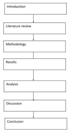
Structure of study
The study has five notable sections namely the introduction, the literature review, methodology, results and findings, and the conclusion. The introduction will provide a basic overview of the topic at hand. This section highlights the aspect of energy detection of signals of unknown nature that also have fading characteristics. The project is also justified in this section and its importance is highlighted.
The literature review section adequately covers previous works that are related to the topic of study. This section attempts to gather knowledge and information from the studies that have been done by earlier researchers. Special emphasis is paid so as to ensure that all borrowed knowledge is relevant and applicable to the topic of study.
The methodology section will highlight the means and approaches used so as to come up with relevant data. The data acquisition methods will also be assessed and analyzed in the methodology section.
The results collected as a result of the study will be highlighted in the results chapter; this chapter will critically analyze all the raw data. This section contains graphs and tables that show the outcome of the study.
The results on the other hand will be analyzed in the discussions section. In this section, the raw data will be assessed and from this data, the researcher will be able to make inferences.
The conclusion is a brief summary of the whole study. However, this section will pay special emphasis on the strengths and weaknesses of the study. From these strengths and weaknesses suggestions on how the study can be improved are made.
Literature Review
Cognitive radio spectrum sensing
Cognitive radio technology is becoming more and more vital in many fields of engineering. The advancement of this technology has brought about new opportunities for cognitive spectrum sensing. This is with the view that a cognitive spectrum sensing system is the driving force of any cognitive radio network (Swamy, 2010).
Spectrum sensors monitor the activities of a cognitive radio system and ensure that the system does result in any unwarranted interferences. There are three basic requirements of any cognitive radio sensor, namely:
- Ø Should have the capacity to detect all transmissions in a particular field
- Ø Establish the source of each transmission in a field
- Ø Be able to communicate and relay data to the central processing unit effectively
A cognitive spectrum sensor is required to be able to sense the presence of any spectrums in a respective field. The sensor is not only required to be able to sense the presence of a spectrum field but should also be able to perform consistently throughout a specified period. This is an important aspect of any effective spectrum sensor as it allows the sensor to establish the various spectrums that exist without providing a window period in which errors could occur. Cognitive spectrum sensors are not required to interfere with any primary signals and thus assume an ‘invisible’ role when in the application (Sampei, 2000).
Cognitive sensors are also required to scan a particular field for any vacant spectrums that may exist. This is in line with a noninterference requirement that cognitive sensor spectrums are required to satisfy. A cognitive sensor is therefore required to migrate from a spectrum when a primary user intends to use the spectrum to a vacant/ dormant spectrum. This property ensures that the cognitive sensor is able to avoid interference with any primary users and thus adhere to this vital requirement.
Early cognitive sensors had difficulties when it came to deciphering and monitoring the type of transmissions received. These sensors were not able to distinguish their own transmissions from external transmissions. With time this limitation has been overcome and most spectrum sensors are able to distinguish between various types of transmissions. The most important distinguishing property of a sensor is that it should be able to distinguish between the transmissions emitted by the primary user from those emitted by itself and those that cause interferences (Prasad, 2003).
There are two main types of cognitive spectrum sensors these are noncooperative spectrum sensors and cooperative spectrum sensors. Noncooperative spectrum sensing is also referred to as the independent type of sense. In this type of sensing the cognitive radio, the sensor is able to map out its own configuration based on the environment that it is in and on the data that has been installed in its central processing unit.
Some scholars argue that the cooperative method of spectrum sensing is the most effective method of sensing in comparison to the noncooperative. However, this type of sensing has its setbacks such as the high cost of installation and of operation. Critics argue that the high investments needed in such a sensing system are often justified by the enhanced performance of the system. This type of sensing system involves the use of multiple sensors that send their data to a central processing unit. In this instance, each sensor is dependent on the other and vice versa. The central processing unit is responsible for analyzing the individual signals from each sensor and defining a mass protocol to be followed by each sensor. The cooperative type of spectrum sensor has been found to be less prone to interference in comparison to the noncooperative ones (Mgombelo, 2000).
There are different types of cognitive radio signal sensors. The choice of an optimum sensing methodology is often dependent on how well the sensor is able to satisfy the various requirements of an effective sensing mechanism. A cognitive radio sensor should be able to measure and analyze all signals in an accurate manner and thus be able to avoid errors in measurements. Errors as a result of accuracy problems often result in the generation of false alarms in sensing systems.
How to prevent a cognitive radio spectrum sensor from detecting its own signals was a problem in the initial development phases of spectrum sensors. This led to the development of timing windows. During a timing window, a spectrum sensor does not transmit any signals and it is at this time that it also takes measurements. These windows allow the effective measurement of foreign signals by spectrum sensors (Mahmoud, 2007).
Spectrum sensors are required to establish all types of signals emitted by the primary user and by other units in a field. This property allows the sensor to be able to distinguish between wanted and unwanted signals in a field. This minimizes the possibility of interferences and other spurious signals from being incorporated into a sensing system.
The sensing bandwidth of a cognitive spectrum sensor is also of great importance. This is because wide sensing bandwidths often result in a lot of noise and interference signals. This is because of the widened area of scope of the sensor. However, a very narrow bandwidth often results in a system that is unable to effectively measure the number of available channels in a system. Sensors with wide bandwidths are often able to gather more data on the available channels i.e. whether they are vacant or not. Such a system is, therefore, able to create a larger list of alternative channels to be used when required. The optimum bandwidth of a sensor is often left to the designer who should weigh the advantages and the disadvantages of a specific bandwidth size (Katz, 2007).
A major challenge that most cognitive spectrum sensor designers face is in ensuring that a system is efficient enough. For a sensor system to be efficient the designer must ensure that the system does not constantly migrate from one spectrum to another. Such migrations happen in instances where most spectrums are occupied and thus force the sensor to seek alternatives. Too much migration may lead to a system becoming useless. The cognitive radio system must be able to adjust together with the sensors as they migrate so as to accommodate the migratory properties that most sensors exhibit.
Cognitive radio spectrum selection
Spectrum selection in cognitive radios is based on the ability of these radios to sense parameters in their environment take action based on these parameters and then make independent decisions. Action involves tuning the sensor while decision involves changing the sensor configurations based on the parameters in the environment.
There are two types of decision making methods that are used by spectrum sensors namely the analytic method and the machine based learning method. With time the machine based learning method has gained more popularity due to its ability to be employed in expert systems and the ability of the sensor to generate genetic algorithms. This also allows the sensor room to learn and generate its own decision making mechanisms. The analytical method is based on simple optimization methods and thus has proven to be an ineffective method especially in large scale operations (Hossain, 2007).
Reinforcement learning in reference to spectrum sensors refers to the ability of the sensors to take account of the occurrences in the environment, make decisions on these occurrences and then keep account of feedback as a result of the decisions made. This type of learning takes the form a circle and ensures that the sensor is involved in an endless cycles of learning and improvement. There are various difficulties that are often faced by sensors in their decision making processes, these are quality and consistency issues of the network users and environmental characteristic such as nature of spectrum availability. For a sensor to be said to have a reinforced type of learning it is required to be able to operate on its own without any external control (Fette, 2009).
Markov decision process
The Markov decision making process refers to a mathematical model that is used in the making of decisions. It uses an analytical form of modeling that is used to modern day reinforcement learning processes. This decision making process is governed by a set of functions that are represented by various letters.
S = a specific set of states
a= a specific set of action/s that occur in the said state
r = the reward accrued as a result of actions in the said state
t = the state distribution function
π = refers to the policy put in place to maximize the reward
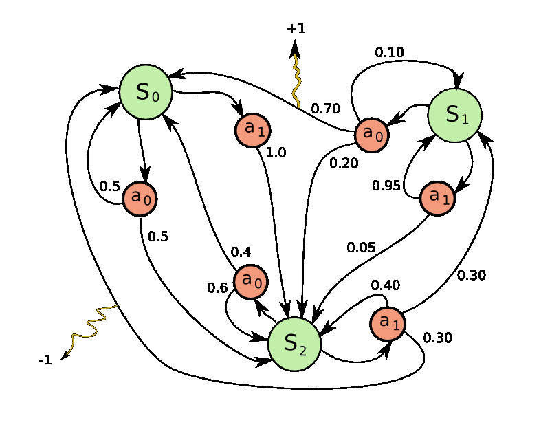
The implementation of the Markov model results in a Markov chain that is able to execute decisions that are relevant to reward and state conditions. This process has two main algorithms which are used in the decision making process
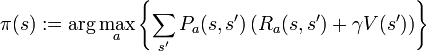
![]()
Where:
P = transition function
R = reward function
V = represents real values
V(s) = total sum of rewards that have been discounted
There is no specified order in which the two algorithms are computed but the algorithm is self correcting and ends up in a common answer. Reinforcement learning has proven successful not only in cognitive radio spectrum sensors but in many fields due to its ability to create optimal conditions for various environments and to be able to generate positive outcome in large environments (Elmusrati, 2010).
In cognitive radio spectrum sensors joint spectrum power selectors are often used. This is mainly in environments that have more than one transmitter. Each transmitter and receiver in the network is also able to select its own suitable parameters and thus each is unique in its own way. In such a system emphasis is put so as to maximize the performance of each sensor while at the same time ensuring that each sensor is able to filter out as much interference as possible (Dulal, 2009).
Below is an outline of initial and final epochs in a joint spectrum power system:
Initial epoch s, spectrums>
Choose a random value labeled r (x,y)
If r < ᴈ
S = random state
S = argmaxs
Final epoch
Start transmissions
At the end of each transmission analyze rewards and implement reinforcement learning
In a cognitive radio system each epoch is often divided into several slots. During each slot the cognitive radio system is able to decide on a certain action and is able to evaluate the rewards of the action. The level of reward from each slot is determined by the characteristics of the transmission. Collision and interference often result in negative rewards as compared to successful transmissions which are regarded to have positive rewards (Bagad, 2009).
Energy control is an important aspect is sensing. This is because each sensor must be able to determine whether its expenditure on energy is as planned. Most cognitive sensors have an inbuilt ability that allows them to calculate their rate of energy consumption. A sensor’s energy consumption is often compared to its expected/ planned energy consumption and then corrective measures taken by the cognitive radio system. This is done as values outside the threshold result in negative rewards that in turn trigger corrective actions though the reinforcement learning system (Arslan, 2007).
A cognitive radio system that has too many negative rewards and is unable to generate positive rewards is identified as faulty and erroneous. This is an important exercise as it facilitates the removal and replacement of faulty cognitive radio systems.
Cognitive radio sensors that employ the use of reinforcement learning have been found to have a higher probability of generating successful transmissions. This is established as a result of experiments that have been conducted on both reinforcement learning and DSA algorithms. After a considerable number of epochs (over one thousand) the reinforcement learning algorithm is able to generate more successful transmissions. The number of successful transmissions is measured by the num be of stationary PU activities in a system. However in low numbers of epochs (below 1000) the number of successful transmissions in reinforcement learning algorithms is very low. This means that this type of algorithm is particularly effective for a high number of epochs (Prasad, 2003).
Detection and false alarm probability in AWGN channels
AWGN sensor networks are networks that have a constant white noise transmission incorporated into the system. Most theories on AWGN do not take into consideration other factors such as interferences, fading, dispersion, non linearity and frequency selection and attempt to gain some insight on the inherent characteristics of sensor networks with respect to white noise only (Sampei, 2000).
The actual source of AWGN transmissions has not yet been fully established and there are many theories as to the exact source of these transmissions. The most credible explanation as to the source of white noise in AWGN networks is that white noise comes from the vibration of particles and atoms of conducting particles in the environment i.e. solar white noise.
Below is the derivation process o the AWGN formula
Zi ~ N (0, n)
Yi = Xi + Zi
I (X; Y) = h (Y) – h (YX) = h (Y) – h (X + ZX) = h (Y) – h (ZX)
I (X;Y) = h (Y) – h (Z)
h (Z) = ½ * log (2 * pie * e * n)
E (Y2) = E (X + Z)2 = E(X2) + 2E(X)E(Z) + E(Z2) = P + n
h(Y) <= ½ * ( 2* pie * e * (P + n))
X ~ N (0, P)
C = ½ *log(1 + P / n)
In the study formula for the calculation of false probability was derived. The probability of detection could also be calculated using this new technique. These two are represented as Pf and Pd respectively. According to the formula:
Pd = Pr (y > ʎ/ H1)
Pf = Pr (y > ʎ/ H2)
The resultant false alarm and detection probabilities are
Probability of detection over fading channels
This type of detection is mainly carried out on Nakagami and Rayleigh channels. The probability of false alarm in this type of detection often remains constant because it is not affected by the signal to noise ratio of the system. However the probability of detection is this setup can be easily estimated. This is done using the below formula.
ƒNAK (γ) = 1 / Γ(m) * (m / Ў)m * γm-1exp(-m/Ў*γ), γ=> 0
and
Where:
m = the Nakagami parameter
Ў = is the total average of the signal to noise ratio
Pd,NAK = The probability of detection in a Nakagami channel
Β = hypergeometric function that is confluent in nature
A1 in the calculation of the probability of detection in a Nakagami channel serves as a representative of a group of calculations. This is used so as to shorten and to simplify the calculation of the detection probability (Vij, 2010).
Nakagami channels
A proper understanding of Nakagami channels is needed so as to be able to devise energy detection mechanisms over these channels. In Nakagami type of envelopes, the resultant power is gamma-distributed. Fluctuations in Nakagami channels can be less in comparison to those of Rayleigh channels when the shape factor of the Nakagami channels is greater than 1.
Nakagami is used to describe the amplitude of received signals after diversity combining of maximum ratio. This is illustrated after a k branch of maximum ratio combining passes through a Rayleigh system and results in a Nakagami system with a shape factor that is equivalent to k. When a Nakagami signal is merged with the k branches this results in an overall signal with a shape factor of m * k. The resultant shape factor is MK (Xiao, 2008).
When Rayleigh signals of identical nature are added to each other they result in a Nakagami model. This is commonly caused by interferences in cellular systems that originate from multiple sources. The Nakagami type of distribution is often preferred as it is able to prepare to match empirical data in comparison to the Rayliegh distribution.
There are various characteristics of Nakagami fading in systems. These characteristics are particularly distinct in the conditions and factors that lead to the development of each system. Nakagami occurs in systems with multipath scattering coupled with relatively large spreads of delay time. A distinct characteristic of clusters in Nakagami is that there are reflected waves existent in the cluster and that have similar times of delay when the delay times happen to be more than the bit time then this results in inter-symbol interferences throughout the different clusters of the system. In such instances, co-channel interferences through Rayleigh fading channels that are incoherent are estimated using multipath interferences (Mgombelo, 2000).
The Nakagami model has been found to be strikingly similar in behavior to the Rician model, as it approaches its mean. Critics however claim that that is not enough evidence to warrant the interchangeable use of both models. This is because the Nakagami model when used instead of the Rician model tends to provide inaccurate results in the tail regions of the distribution. Bit errors mainly occur during cycles of deep fading and thus the Nakagami model has been found to be lacking as its performance in such times is measured by the probability distribution tail.
The Nakagami model has been found to respond poorly when used in approximation in instances where the fades are deep that causing the error rates to differ greatly. The common misconception that the Nakagami model is able to completely replace the Rican model has resulted in multiple errors in the calculation of cognitive radio parameters. Proper understanding of Nakagami type of fading is needed so as to be able to carry out proper estimations on the energy content of unknown signals. Below is a chart of the differences between these two models in fading channels (Katz, 2007).
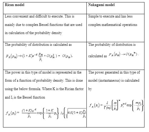
The close form probability of detection formula in the Nakagami model are written as
However this equation is often very complex and thus cannot be used in the direct calculation of the probability of detection over the Nakagami channels. Therefore this primary equation is further simplified so as to make it more convenient for practical applications.
The second term in the primary equation has been simplified so as to generate the second equation. In the second equation it can also be noted that there is a notable difference in the expression A1
The validity of the above formula is tested using mathematical simulations. The simulations generated by MATLAB show that these expressions are correct and consistent. The graphs showed that the simulated and theoretical values generated were similar. This proves that these formula are valid and that they could generate accurate results in Nakagami approximations (Bagad, 2009).
Square law combining over Nakagami channels
Energy detection of primary signals is often a difficulty experienced when trying to estimate the energy content of these signals as they go over Nakagami channels. Nakagami is the most common type of fading that is experienced; involves the addition of the individual outputs of each square law device and then developing a final decision statistic. A Rayleigh system with the diversity branches that are equivalent to m multiplied by L are equal to a Nakagami system of m in an L diversity system; square law combining (Rappaport, 2002).
When designing a cognitive system it is important to have a clear outline of all primary and secondary users that exist in the system. Primary users are the most important users in a system and it important to ensure that they do have any conflicts with secondary users. For the efficient use of a cognitive system to be achieved it must be ensured that secondary users utilize the idle proportion a system and that this utilization does not cause any interference to the primary users.
When a system exhibits fading properties it becomes extremely difficult to ensure that the secondary users do not interfere with the primary users. This is because of the shadowing effects of fading that undermine the sensing abilities of a cognitive radio. Cognitive spectrum sensors and diversity systems are often implemented so as to improve the accuracy and performance of such a system (Smith, 2006).
There are many formula and techniques that are used in diversity systems such as selection combining, equal gain combining and maximum ratio combining.
The use of square law combining was proposed by a scientist named Digham who was able to derive equations for the calculation of probability of detection and probability of false alarm using diversity systems. The diversity systems used by Digham were relatively simpler forms of diversity systems that employed square law combining and square law sensing (Swamy, 2010).
Square law combining in Nakagami channels is similar to other types of square law operations in the mode of its formula generation. The principle formula for this type of operation is:
Where m represents the Nakagami parameter and k the square law devices. The signal to noise ratio is represented by ɣk

In instances where m can be said to integral then the below is developed
Detection of primary users without diversity
This type of detection uses a square law device and has a finite time integrator incorporated into it. This technique makes use of hypotheses of binary nature. Below is a representation of the implementation of binary in this detection method.
H1 this hypothesis states that there is no signal
H0 this hypothesis states that there is a signal present
h is the channel gain that is instantaneous
r (t) is the received signal
s (t) refers to the primary signal
n (t) additive zero mean of white noise; Gaussian noise
H1 : r(t) = h(s) t + n (t)
H2 : r(t) = n (t)
For the determination of the real primary users to be possible a Y decision parameter is devised. The statistic is calculated as shown below:
No represents the one sided noise signal, W represents the bandwidth of signals, T represents the time interval in which observation of frequencies was carried out and N is the number of sampling points in each observation that was carried out (Hossain, 2007).
Square law combining in AWGN channels
Square law combining in many applications is used in AWGN channels. This is because it has the ability to enhance the sensing properties of a cognitive radio system. The decision statistic in this setup has been found to follow chi square distributions that are central in nature. This is with respect to the degrees of freedom of the variance (Vij, 2010).
The probability of false alarms in AWGN channels is calculated by the below formula
This equation is further modified since under the H1 hypothesis, the decision variable used in the above equation has a chi square distribution that is non central in nature. A parameter to cater for this property of non centrality is derived and then incorporated into the above equation.
The incorporation of the parameter due to non centrality results in a change of the equation to
The above equation represents the final formula that is used in the approximation of detection probabilities in AWGN channels
Square law combining in a Rayleigh channel
In the square law combining of this type of channel the PDF of the system is often calculated using the below formula
Based on the above formula, the average of probability of detection in Rayleigh channels can be calculated.
Other forms of the formula could be created. Examples include closed form formulas that can be produced from the above equation by replacing key parameters such as m with L and
![]()
The main formula that is used to calculate the probability of detection in Nakagami channels is
The performance of a square law combining system over a Nakagami channel is done using receive operating condition curves. These curves are plotted with respect to two and four diversity branches. Various values of m are used so as to facilitate proper plotting and evaluation of different parameters. Vales of m such as 1, 2, 3, and 4 are used. It is however noted that the spectrum sensing abilities of the system tend to perform better with higher values of m. It was noted that 4 had the highest sensing abilities compared to 1 which had the lowest. This proves that the Nakagami parameter has a significant influence in the spectrum sensing abilities of a system. The rate of change of sensing abilities was found to increase as the system was moved from parameter 1 to parameter4. This means that there is a greater improvement in abilities as the system moves from 1 to 2 in comparison with 3 to 4 (Mahmoud, 2007).
The diversity branches have also been found to affect the sensing abilities of a Nakagami channel. This is particularly true when there are a larger number of diversity branches in the system.
The Nakagami parameter has an effect on the sensing abilities of a system. The magnitude of this effect is also dependent upon the number of diversity branches. The parameter m has been found to have greater effects on the spectrum sensing abilities of a system if there exists a higher number of diversity branches in the same system.
Diversity branches have been found to have great influence in the sensing abilities of a spectrum sensor. This ability is also directly proportional to the number of diversity branches in the system. When a diversity system is not in use the formula for the detection probability is much simpler and easier to use. Closed form formulas are used whenever diversity branches are employed in Nakagami systems (Arslan, 2007).
Methodlogy
The techniques and methods used in the study were carried out in an attempt to prove the effectiveness of several energy detection techniques and mechanisms. These techniques were proposed by Digham together with his fellow scientist. Digham claimed that he had a method that could be used to effectively approximate the energy content in unknown signals (Bagad, 2009).
The key characteristic of the experiment was that the signals had to pass through fading channels. The Nakagami and Rayleigh channels were simulated so as to measure the effectiveness of the proposed methods.
In preparing the scope of executing the project a secondary goal of the experiment had to be noted. In the studies a relationship between the diversity branches of their relationship to probability of detection had to be established.
Various aspects of energy detection in fading channels will be assessed. These are energy detection under varying parameters such as Nakagami m and divert branching. The study proposed that detection abilities in a cognitive radio system can be enhanced by varying the number of diverse branches (square law combining and selection)
For the study to be able to be well analyzed models of a cognitive radio system are needed so as to be able to get practical readings. Models are effective methods in which spectrum sensing can be well analyzed. However practical tests have many constrains such a time, cost and the fact that they are prone to errors makes them less popular. Modeling and testing software such as MATLAB are used. In this study MATLAB will be used to simulate the theoretical performances of the systems proposed in the study. This theoretical performance will also be compared to the simulated performances. The use of MATLAB in the study will save time and cost and reduce the number of loopholes that could be a source of errors in the study. A MATLAB package version 7.11 will be used in the study to analyze the formulas.
The study will cover low pass and band pass filters but more emphasis will be placed on the band pass filters. In practical testing the energy will be measured and detected by a sensing unit. This unit will also quantify the various levels of energy that it receives. Records of these will be kept so as to be used in the preparation of the resultant charts.
A problem in this type of experiment is on how to measure a signal that has passed through the band pass filter. Efficient measurement of this is important and it is the only way the energy of the wave could be quantified. The filtered signal is squared and then integrated with respect to the prescribed time interval so as to create a measure of the energy that is potent in the wave (Fette, 2009).
There are various parameters that will be measured in the study. These will be beneficial in determining the validity of the study. Below is a table that shows the different parameters measured and their descriptions.
Results and Findings
Introduction
The study findings determined that communication technology relies on capacity for energy detection of unknown signals that might be transmitted through fading channels. Different approaches have been determined to form basis for approximation of energy detection of signals transmitted into fading channels. The capacity to measure energy content of unknown signals in fading channels has capacity to inform policy development on strengthening of signals through energy management. The findings of this study demonstrate rationale for approximation and generation of simulations of signals through energy detection. This is based on formulas and principles of simulation of signals transmitted via fading channels. The results provide analysis of two types of fading channels namely the Nakagami and Rayleigh. Use of mathematical representation is meant to determine energy content in the fading channel systems. The simulations results demonstrate relationship between theoretical values and observed practical values based on energy detection formula for the signals transmitted over fading channels. The results further quantifies validity construct if the formulas for detection of energy content of signals transmitted over fading channels namely Nakagami and Rayleigh.
The simulation results present individual detectors namely the sequential detector and truncated sequential detector, the Rayleigh channels and log normal shadowing channels and its roles in cognitive radio spectrum sensing and selection. This is based in capacity to determine and propose applications of square law combining and square law selection. The study seeks to determine performance of block based detector that is transmitted over a Rayleigh channel and influences of variability of bandwidth on different average received SNR as well along normal shadowing river various tome bandwidths. There is requirement for understanding of preset values like SNR and PD and can contribute into ability to improve detection performance through use of square law combining and square law selection.
The Nakagami and Rayleigh signal simulation environment
Use of the AWGN simulation environment
The use of the AWGN simulation environment was structured to utilize a QPSK type of channel. The QPSK channel was adopted as best alternative for determination of unknown signals whose bandwidth is greater than zero. By taking mathematical notations
Es/No [is assumed to represent relationship between Primary Signal Energy with respect to Noise Energy. In the event Es is used to denote Energy, then the Noise Power (No) spectral density is represented by mathematical notation
Es = Ps/R …..Equation one
Where No = Pn/R ….equation two
From equation one and equation two,
Pn (is considered to represent average noise power, R represents Rate of symbol and Ps represents Signal power per given symbol. If a ratio of Es and No is sought, the outcome is represented by equation three
Es/No = Ps/R * R/Pn …equation three
This translates into Es/No = Ps/Pn ….equation four
If equation four is rearranged by making Pn the subject of the formula
Pn = Ps/[Es/No] …..Equation five
In the event Es/No is expressed in terms of dB equation four (Es/No = Ps.Pn) can be rewritten with Pn as the subject of the formula namely
Pn = Ps. 1/[10 (Es/No)/10] ….Equation six
The Gaussian Noise has been documented in literature to be equally distributed. As a result, average power per given dimension can be expressed in terms of in-phase and Quadrature-phase channels which could be represented by equation seven
Attn= Square root of [0.5Pn] …..Equation seven
By defining energy content per given specified sample, and identifying sensing time as time T, the energy per given specific sample based on Nyquist rate sampling could be defined by
PsT/2WT = Pn/2W …………..equation eight
Where Pn is the noise power, T is time in seconds; PnT is energy within T seconds period.
In the event equation seven is divided by equation eight, we end up with (Ps/2W)/(Pn/2W) which translates into Ps/Pn; thus
Ps/2W)/(Pn/2W) = Ps/Pn ……equation nine
Equation nine is similar to equation three
The analysis of the fading channel and its characteristics
The fading channel arises when the received signal by a sensor undergoes attenuation process that is characterized by a fading factor denoted by α. Upon passing through a fading channel, a fading channel is perturbed by AWGN. The instantaneous signal to Noise ratio could be mathematically be represented by
γ = α2Es/No …….equation ten
Based on equation ten (γ = α2Es/No), it is possible to derive the average SNR per symbol which can be represented by mathematical notation represented by equation eleven
…equation eleven
The simulation channels
The study relied on the use of a non selective Rayleigh fading channel. In Non selective fading channel, the factor for the fading of the channel signal is assumed to be constant within a given symbol period. It is also assumed that the fading factor for the non-selective fading channel has capacity to vary from one symbol to another. The second channel that the study investigates its cognitive radio spectrum sensing and selection is the log normal shadowing channel. The log normal shadowing channel is assumed to have a standard deviation of 6dB. In literature, statistical analysis has determined that standard deviation of log normal shadowing channel lies between 2dB and 14 dB.
The major parameters used in simulations
The simulation procedure dependent on two main variables or parameters for investigating spectrum sensing and selection, with regard to non-selective Rayleigh channel and log normal shadowing channel. The first parameter for simulation was identified as the Average Number of Samples (ANS) represented by n where n is a variable that is a function of decision making process. The sensing time in the case of sequential detector is represented by mathematical notation denoted by equation twelve n= summation of required samples in every simulation loop ÷ number of simulation loops that are used.
Based on Average number of samples, for every given simulation that is determined and investigated, the main transmitter sends a specific number of samples. The minimum number of samples that are transmitted during every simulation should at least be greater than the number of samples that are going to be used in making a decision. This implies, if the number of samples that will be transmitted is equal to the number of samples that are needed to make a decision, and then it means, the number of samples for making decisions are not adequate. This is because the number of samples that are transmitted in a given simulation process is independent of the performance capacity of the detector irrespective of whether the detector is sequential detector or truncated sequential detector. What matters and affects decision making capacity of a detector is the decision interval. The second main simulation parameter is termed as average percentage saving (APS). APS of a detector (primarily sequential detector) is represented by mathematical notation thirteen
PS = [1-(n/Nfss] × 100%
The denominator [Nfss] denotes the number of samples that are needed at an instant in order to make it possible for a block energy detector to attain a specified performance level.
Implementing individual sensing
The capability of energy detection in a fading channel and log normal shadowing channel are dependent on quantity of SNR received as well as the interval of decisions. in application of MATLAB modulation, its possible to compare signal energy over the decision interval as a function of the threshold and block based energy detector in order to form basis for decisions. The threshold of energy detector for a Rayleigh fading channel has equivalent properties as the AWGN channel. Any deviation could be achieved through normalization to ensure equivalence in terms of preset PFA values and decision intervals.
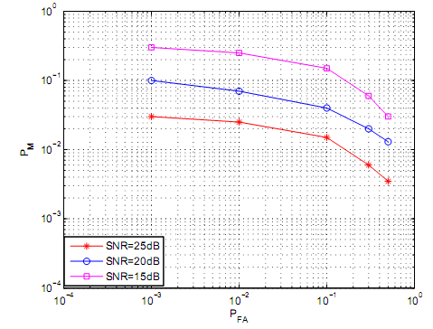
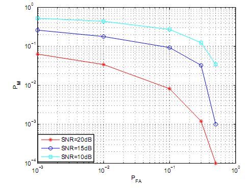
Modeling of a Rayleigh channel could be achieved through Jakes model. This forms basis for capacity to describe performance of a detector based on ROC. The ROC values could then be plotted as a function of PM and PFA. If for instance, the main transmitter transmits a hundred samples for every simulation loop, then it implies, a hundred samples could be considered as arbitrary choice as represented by figure 5. In the case of figure 5, the decision interval has been set at ten samples which mean energy detection takes in the first ten samples and makes decisions for every simulation loop. After a decision is made, the simulation loop ends and the simulation loops starts all over again
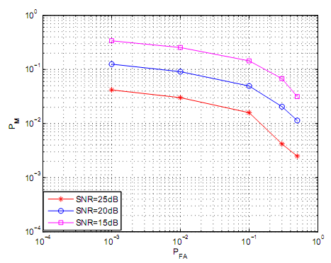
Figure 5 illustrates complementary ROC (Receiver Operating Curves). The ROC was realized on Rayleigh channel following varieties of average received SNR. The decision interval was fixed into a constant in order to determine variability of received SNR. In figure 5, the PFA and decision interval were primary variables that were used to set the threshold. Based on the PFA and the Decision interval, the primary objectives was to determine the variability of the values of the PM. Figure 5 findings illustrates that PM is indirectly proportional to PFA hence as values of PM decreases, the values of PFA increases. Based on figure 5, it could be deduced that values of PFA influence on the threshold. As a result, large values of PFA result into very small threshold which translate into small values of PM. From figure 5, it is evident that as for a specific value of PFA, the values of PM decrease inversely to corresponding increase in values of SNR. The main reason for the increase is that if a primary signal has a high average SNR, the corresponding PM would be low if the PM value is fixed and constant. Figure 6 and figure 7 provide more illustrations on variability of PM, SNR and PFA for complementary ROC. This is based on Rayleigh channel fading. In figures 6 and figure 7, the decisions are based on 6 samples for figure 6 and 20 samples for figure 7.
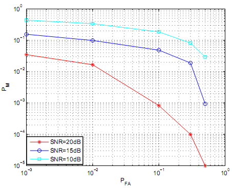
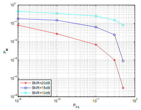
Figures 8, figure 9 and figure 10 demonstrate variability of complementary ROC for the case of a log normal shadowing channel. The standard deviation of the log normal shadowing channel is set to 6dB. The 6dB was set for varieties of SNR and decision interval. The magnitude of decision interval for figure 8 was set at 6 samples, figure 9 at ten samples and figure eleven at twenty samples. Based on simulation data on log normal shadowing channel, the values of PM decreases a s PFA increases hence demonstrating that PM and PFA are inversely proportional. It is also evident that if PFA is fixed, PM and SNR are inversely proportional.
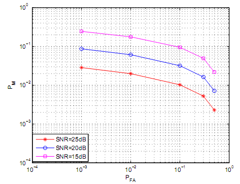
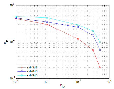
Figure 11 illustrates log normal shadowing channel energy detector and level of its performance. Different values of standard deviation shadowing are illustrated and presented. The sample size for decision interval for the figure 11 is ten while the average observed average SNR is 10dB. Base don figure eleven, it is evident that as PM rises, the value of the standard deviation increases which implies the relationship between the PM and the standard deviation demonstrates positive correlations.
The role of the sequential energy detection
The sequential detection was determined in basis of two major elements namely the average number of samples required and the distribution of quantity of required samples for decision making. The primary transmitter is based on MATLAB modulation. The quantity of samples that were required in order for the sequential detection to execute decision making was based on random variables which had capacity of assuming small to large values.
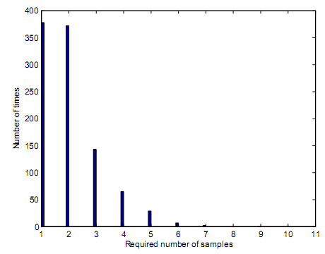
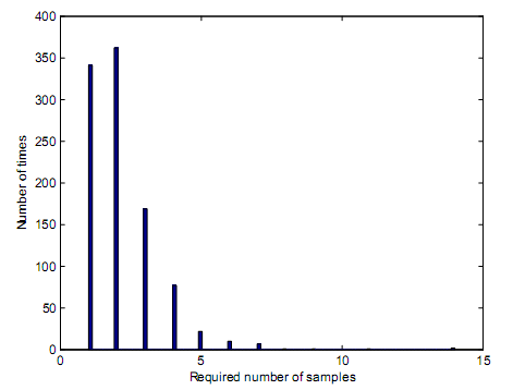
Based on variability of the sequential detector, the primary transmitter should demonstrate capability to transmit 500 samples. The samples that were transmitted in every loop of simulation commences when the simulation loop begins and ends when a decision is reached based on the preset PM and PFA values as well as truncation points. The preset truncation point is the number in which the simulation decision should be made to result into termination of simulation loop. Figure 12 demonstrates sample distributions in case of a sequential detector when the main signal has AWGN characteristics. For instance, in figure 12, the sequential detector requires 5 samples to come up with a correct decision. Analysis is made on simulation loops that result into a decision making. For figure 12, the preset PD is 0.99. by carrying out analysis on correct decisions, and establishing 989 simulation loops are correct out of 1000 simulation loops, then it means the PD is 0.989 which is represented as 0.99 in two decimal paces. Figure 13 demonstrates distribution of number of samples that are proposed.
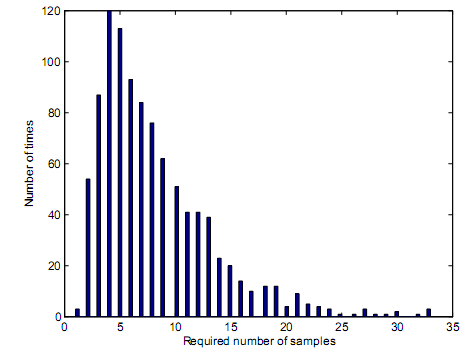
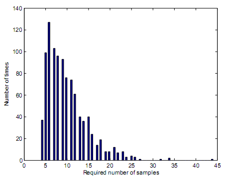
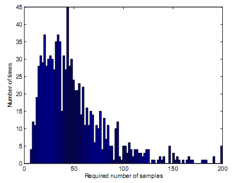
Figure 13 demonstrates a sequential detector that has AWGN characteristics. The signal has no main signal that is present hence preset PFA is 0.01 if the preset PFA is 0.01. Upon finding 992 correct simulation loops that might have contributed into correct decisions, it implies, PFA value is calculated to 0.008 which is equivalent to 0.01. As a result, the required number of samples would be 9.92 as illustrated by figure 13. Lack of primary signal results into inability to determine the impacts of log normal shadowing or received SNR as illustrated by figure 14 and figure 15. this is further illustrated by figure 15, figure 12 and figure 14.
Based on figure 16 and figure 17 the required number of samples that were needed to contribute into decision making was found to be 7.85 and 6.18. The values in figure 16 and figure 17 demonstrated that increasing values of PD has effect of increasing the number of samples hence paving way for direct proportionality.
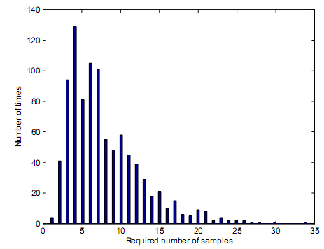
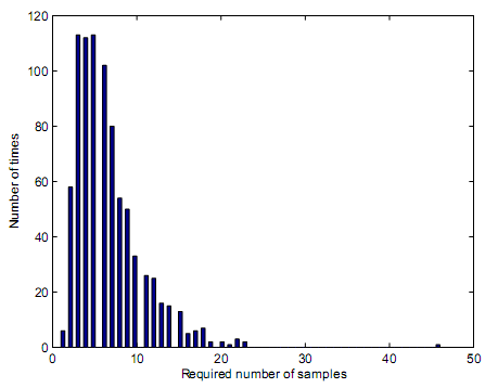
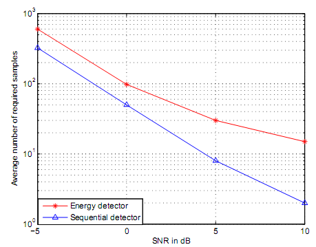
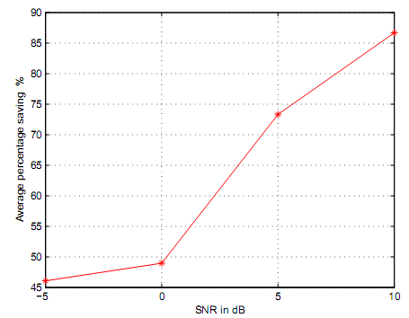
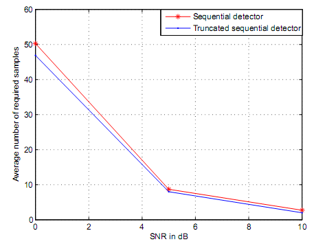
Figure 18 and figure 19 are based on AWGN channel where preset values of PD and PFA were 0.99 and 0.01 for the sequential detector. The required samples for block based energy detector were set at different truncation points. The simulation results based on figure 18 demonstrated that sequential detector has capacity to reduce the number of samples that are required to make decisions by 45-85%. This positions sequential detector to have capacity to detect primary signals fast and at higher detection accuracy compared to truncated sequential detector Figure 18 illustrates average percentage saving that could be achieved by sequential detector. For instance if the SNR is 0dB, it implies, there could be a saving of 48% of the required number of samples following use of a sequential detector. Average power saving based on figure 15 has capacity to result into variability of SNR thus from lo to high SNR values.
Simulation results of a truncated sequential detector
The number of the required samples that should be used to achieve a truncation point should be minimal. Based on literature, the required number of samples that contribute into making of a decision is based on random variables which may take either low or very high values. Determination of the maximum optimal number of samples that are needed to make a decision is important element in cognitive radio spectrum sensing and selection. As a result, truncated points and truncated values should be based in terms of truncated sequential detector with respect to the number of samples and any preceding degradation in terms of performance that may result after truncation. The literature on cognitive radio spectrum sensing and selection affirms that the minimum samples that are needed by a truncated sequential detector ought to be lower than that of sequential detector.
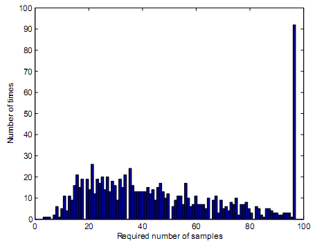
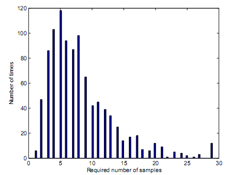
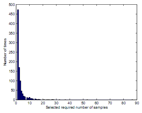
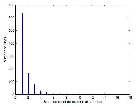
Decision rules depend on square law combining and square law selection. Since truncation point represents the total number of samples that result into equivalent same performance with block energy based detector, figure 16, figure 17, and figure 18 have demonstrated the number of samples that could result into a truncation point with respect to equivalence of similar performance between truncated sequential detector and sequential detector. The preset values for figure 16, figure 17 and figure 18 were present to PD of 0.99 and PFA of 0.01. The truncation point for figure 16 is at 97 which means, simulation loops made decisions after 97 samples were received. This explains why the rightmost bar on figure 16 is widest. Although the truncation point occurs at a very low value of SNR, the number of samples needed to make a decision ought to be 97 or above. At the same time, figure 17 and figure 18 demonstrate their truncation points occur at 29 for figure 17 and 14 for figure 18 respectively.
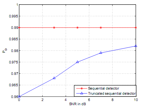
Based on figure 20, figure 21, figure 22 the average samples that were required were 46.89 for figure 20; 8.02 for figure 21 and 2.01 for figure 22. The simulation results demonstrated that the average number of truncated sequential detector was lower compared to the required samples for the sequential detector. This is based on bounding of the number of the samples. Figure 20, figure 21 and figure 22 simulation results demonstrates that average number of samples decreases if the value of SNR received is high. These trends are further illustrated by figure 23. By induction, it is possible to conclude that the performance of a truncated sequential detector is lower compared to performance efficiencies of a sequential detector. The truncation points for PD that was achieved post simulation through MATLAB are demonstrated by figure 24. Figure 24 demonstrates degradation of PD with regard to preset PD values. The PD in figure 24 was preset at 0.99. PD of 0.99 as preset in figure 24 is the design value for the sequential detector.
The log normal shadowing channel and truncated sequential detector
After application of log normal shadowing channel with truncated sequential detector, the standard deviation was set at 6dB for all simulation lops that were conducted. For every simulation loop using MATLAB, the number of transmitted samples was extended to the order of 2000 samples. Based on figure 25, it is possible to deduce that a higher number of samples are utilized in a log normal shadowing environment before truncation process. Figure 26, figure 27 and figure 28 demonstrate the distribution of the samples that were required for truncated sequential detector with respect to log normal shadowing channel. In the case of figure 26, figure 27 and figure 28, the PD was preset at 0.99 (the design value of sequential detector) and PFA set at 0.01. in figure 26, figure 27 and figure 28, the average received SNR were represented by 5dB for figure 26, 10dB for figure 27 and 15dB for figure 28. The truncation point for figure 26, figure 27 and figure 28 were set as block energy based detector in which the sample quantity achieved equivalent performance compared to sequential detector. Figure 29 demonstrates average number of samples that were needed to decrease if the average SNR values were increased. However, the degradation was observed to be minimal if the SNR values increased to very high values.

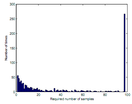
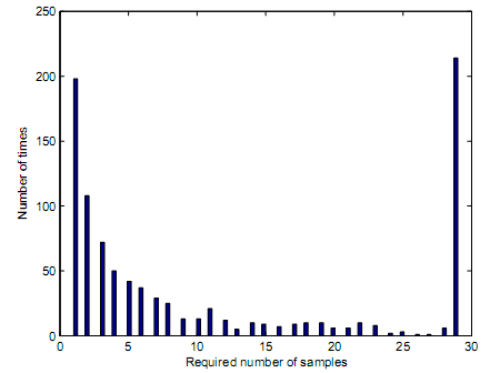
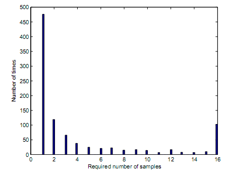
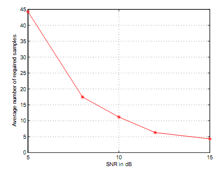
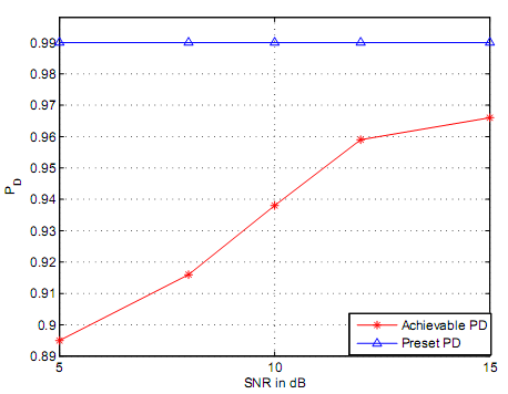
Figure 30 illustrates performance degradation of truncated sequential detector. The performance of sequential detector is compared with performance of truncated sequential detection through application of log normal shadowing channel. Based on figure 30, the present values of PD and PFA are determined as 0.99 and 0.01 respectively. Based on figure 30, it is not possible to realize a preset PD cannot be realized or achieved if truncated sequential detector is used. Based on figure 30 truncated sequential detector loses 0.1 of its performance if average SNR is pegged at 5dB while loses increase loses of performances are to the order of 0.02 if SNR is pegged at 15dB. This can result into a conclusion that as PD is gradually increased as SNR varies decreases.
The influence of square law combining and square law selection
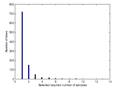
The results of square law combining and square law selection were conducted through use of a MATLAB modulation. In these simulations, the primary transmitter was assumed to have capacity to transmit five hundred samples for any given simulation loop. The square law combining and square law selection are applied at the fusion center. The MATLAB modulation was structured such that it was capable of managing hidden terminal problems. The log normal shadowing channel that had a preset standard deviation of 6dB was used. Upon application of the square law combining and square law selection different outcomes were observed as represented by figure 31, figure 32, figure 33 and figure 34. in each of the figure 31, figure 32, figure 33 and figure 34, the notation represented by letter X is used to represent the quantity of samples that were used at a given fusion center in any specified simulation loop. The letter Y represents frequency of the samples that were required in a thousand possible simulation loops. It is inductively determined that average received SNR as a function of PD and PFA are equivalent for the individual sensors that were investigated. The average SNR were determined at 5dB while PD and PFA were preset at 0.08 and 0.01. The figures 31, figure 32, figure 33 and figure 34 had individual sensors were 2 for figure 31; 4 for figure 32; 6 fort figure 33 and 8 for figure 34.
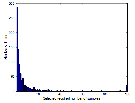
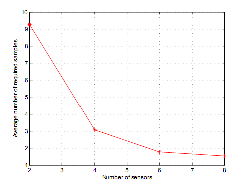
Figure 27, figure 28, figure 29 and figure 30 were determined to have had an average samples represented by 9.27, 3.11, 1.92 and 1.53. Figure 35 illustrates the average values of figure 27, figure 28, figure 29 and figure 30. Based on figure 35, it can be deduced that average number of samples that are needed to make a decisions at a given fusion center decreases as the number of individual sensors increases hence demonstrating an inverse proportionality or relationship between the average number of samples and number of individual sensors. By induction, it can be said that as the number of the individual centers increases, the final decision hat are made are arrived at a higher rate by the fusion center. It is noteworthy that truncated sequential detector has no application with respect to square law combining or square law selection. This is because a fusion center makes decisions based on individual results. Based on figure 35, it is possible to lower the number of samples that are present at the fusion center if the number of individual sensors is proportionally increased. As a result, any requirement for truncation should be carried out at the individual sensor level. This has capacity to decrease performance losses that could result from truncation.
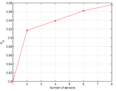
Based on figure 36, the performance of square law selection and square law combining increases if the number of the sensors used increases and vice versa. Figure 36 illustrates that average received SNR as a function of preset PD and PFA are equivalent for different applied sensors. Figure 36 demonstrates the outcomes were achieved at a SNR value of 5dB and further that PD and PFA had preset values of 0.8 and 0.01 respectively. Figure 36 demonstrates that performance of square law combining has higher better outcomes compared to individual unit sensing. This is because, as figure 36 demonstrates, the performance increases as number of sensors increases which demonstrates a direct proportionality.
The relationship between soft and hard decision combining
The capacity for achievement of hard or soft decision depends on exploitation of values of square law selection and square law combining that form basis for adoption of a cooperative approach. Square law combining results into forwarding of individual entities into a fusion center in form of signal energy or likelihood ratio. The forwarded parameters from the sensors form basis for decision making process. Individual entities of a sensor lack capacity to make independent decisions hence its primary role is to collect and forward information regarding a signal. Square law selection adoption results into a scenario where individual sensors make local decisions that are forwarded to the primary fusion center for interpretation and further decision making. As a result, the sensors are entitled to make local decisions which are not the case as in square law combining. This forms basis for hard decisions which means increased demand on energy.
Conclusion
Introduction
This section reports on whether the study achieved its goals and objectives with regard to determination of cognitive radio spectrum sensing and selection. The section reports on simulations results and mechanism the simulation results contribute into determination of rationale for cognitive radio spectrum, cognitive radio spectrum selection, application of square law and square law combining and capacity for energy detection of unknown signals over multi-path channels. The section further reports on rationale for cognitive radio spectrum reduction of time sensing and selection through sequential signal detection. This section proposes on cooperative schemes and individual detectors as functions of Nakagami and Rayleigh channels respectively.
The simulation results demonstrated that Rayleigh fading channel could be employed in modeling of small scale fading environments. The results determined that log normal shadowing channels has application in large scale fading environments. This implies, Rayleigh Fading channel and Log normal shadowing channels are size dependent and applications are size dependent. Log normal shadowing channel and Rayleigh fading channels applications in analysis and simulations were determined to influence on spectrum scarcity. The simulation results demonstrated that problems characterized by spectrum scarcity are managed through dynamic spectrum access. The simulation results demonstrated that cognitive radio spectrum sensing and selection forms basis and foundation for attainment of dynamic spectrum access which is dependent on cognitive radio capabilities as a form of CDR.
The simulation results demonstrated that spectrum sensing contributes into capacity to identify through detection of signal energy of a primary signal that is present in a noisy environment. This is because a spectrum sensing presents signal detection problems in multi-environments or where noisy signal environments are dominant. The problems associated with signal detection problems could be managed through adoption of signal detectors namely, utility of a matched filter, use of energy detector and use of feature detector though they are limited by fixed sample size systems. Based on simulation results, the potential differences provide foundation for determination of sensing time. The simulation results established that cooperative sensing could be used to enhance signal energy detection that could arise from capacity for increased accuracy level of energy detection. The simulation results further demonstrated that cooperative sensing has capacity to decrease sensing time as well as manage problems associated with hidden terminal technical deficiencies. The simulation results further determined that reduction of sensing time is important functional element for the cognitive radio systems.
The simulation results demonstrated that through sequential testing of cognitive radio spectrum, the flexibility of sensing time is increased. The simulation results further demonstrated that PD and PFA should be set initially before carrying out testing. The rationale for energy detention of fading channels transmitted over fading channels namely Nakagami and Rayleigh contribute into capabilities for sequential detector to make independent decisions following recipient of a sample of signal either as individual signal or grouped signal in a multi-channel or signal environment. Sequential detector preferences were based on necessity to decrease the sensing time subject to influence of shadowing environments. As a result, minimal time was reported as opposed to average of the energy detector. The simulation results further determined that sensing time could further be decreased through use of sequential detector. This helps to manage performance degradation that is associated with shadowing environments.
The results of simulation determined that square law combining and square law selection principles have greater role that they play in cognitive radio spectrum sensing and selection. The simulation results determined that sensing times and sensing frequencies result into different energy detection capacities based on log normal shadowing channels. The simulation findings paved way for determination that sensing frequency and sensing times could be decreased or increased. Based on simulation data, the energy detector performances for the signals involving fading channels and log normal shadowing channels depended on two main factors namely time-bandwidth and received SNR. The simulations results established that post application of sequential detector on the AWGN channel varieties of Energies were detected at a shorter sensing time and sensing frequency. This implied that sequential detection required lower average sensing times and sensing frequencies compared to energy detector at the same signal performance which resulted into sequential detector having a higher advantage in terms of sensing times and sensing frequency. The simulation results demonstrated that sequential detector has capacity to decrease sensing times to 80-85%. The results of simulation further established that if the values of the SNR were increased the sequential detector required samples for equivalent performance decreased proportionally. The findings further determined that simulations were dependent on initially system set values for PD and PFA.
Simulations results following application of truncated sequential detector on the AWGN channels however provided different findings. The truncated sequential detector, as opposed to sequential detector, was found to have higher capacity of decreasing sensing times and sensing frequencies to the order of 50-60%. However, independent simulations determined that truncated sequential detector was not significant given that the value of SNR was extremely large. This paved way for application of truncation on the sensing time in order to determine its relationship with different values of SNR. Similar results and findings determined truncation didn’t have any significant impact on the sensing time if the value of SNR was high. This therefore calls for adoption of minimal values of SNR.
The simulation results determined that application of truncated sequential detector on the log normal shadowing channel has impact of elevating sensing time which results into sensing and selection disadvantage. However, the simulation established that the log normal shadowing channel has a range of samples that could support capacity for reduction of sensing time which brings about functionality deficiencies. The findings on log normal shadowing channels further demonstrated that the management of the sensing time increase as SNR increases and vice versa. Simulation data that sought to determine performance degradation arising from truncation demonstrated that the Nakagami and Rayleigh channels demonstrate superior performance under sequential detector as opposed to truncated sequential detector if SNR contribution is not accounted for as a determinant of performance degradation. However, if the SNR contribution was towards performance was integrated; the simulation demonstrated that the performance of Nakagami and Rayleigh channels improved with truncated sequential detector demonstrating higher superior performance as opposed to sequential detector.
The simulation results further illustrated that use of square law combining and square law selection had impact of decreasing sensing time subject to utility of long normal shadowing channel. Based on this data, it could be argued that the sensing time of a detector could be enhanced through increase of the number of sensors. The data supports hypothesis that performance of detection increases as the number of sensors measured in terms of unit are increased. The simulation results demonstrated that square law combining and square law selection supports a hard decision rule that is dependent on a lower bandwidth. A decreasing bandwidth has capacity to contribute into decreased energy detection hence incapacity for improvement of signal energy sensing. The simulation demonstrated that use of soft decision rules supports larger bandwidth. The higher decision rules are based on utility of fusion rules which puts more demand for less bandwidth. Based on the simulation results, soft decision rules as a function of square law combining and square law selection were established to demonstrate better outcomes as opposed to hard decision rules. With regard to individual sensor on Nakagami and Rayleigh channels, the simulation results demonstrated that soft decisions rules have capability to improve on fusion center potential for detection through determination of individual signals. The simulation results demonstrate individual sensors perform sequential testing. The tests results of energy sequential tests are logged on as likelihood ratio to the fusion center. The analyses that are carried out at the fusion center are based on individual sensor signals that first arrive through use of First In-First Out (FIFO) principle. This relies on bandpass filter. The filter is utilizes at front end of energy detectors. Detection arises from capacity to identify signal bandwidth which is dependent on capacity and functionality for wideband spectrum sensing scheme. Wideband spectrum sensing scheme has capacity to elevate bandwidth. Through adaptive approach, cognitive radio spectrum sensing and selection optimizes on varieties of cognitive radio environments. The simulation results demonstrated that cognitive radio spectrum sensing and selection has capacity to contribute into increase spectrum access opportunities which improves service quality for the end users without influence on the network. Rayleigh channels and Nakagami channels were determined to have capacity to be modeled through Gaussian distribution to contribute into avoidance of interference challenges associated with cognitive radio spectrum sensing and selection. The simulation results demonstrated capacity for radio frequencies incapacity to conduct sensing and transmission simultaneously. Incapacity for performance of sensing and transmission at the same time decreases transmission opportunities and affects service quality of end users. Improvement therefore ought to be made to ensure capacity for sensing, selection and transmission of radio frequencies are conducted and performed at the same time. Improved sensing and selection of cognitive radio spectrum therefore has capacity to contribute into management of spectrum efficiency challenges. Thus, cognitive radio spectrum sensing and selection should contribute into adoption of a framework and structure that optimizes on energy detection of unknown signals and sub-bands frequencies that are vacant. Thus, improved energy detection of vacant sub-bands has capacity to contribute into management of spectrum interference sensing constraints hence capacity for enhancement of sensing capacity. The capacity to exploit efficiencies of vacant sub-bands and unknown signals based on energy detection could contribute into development of multi-user and multi-environment functionality environments for cognitive radio sensing and selection with increased interference sensing constraints management.
Proposition for future work
The simulation results identified four key areas that were beyond the scope of the objectives of studies on cognitive radio spectrum sensing and selection. The simulation results were not conclusive on channel performance efficiencies of a sequential detector and truncated sequential detector hence this requires further research to quantify the performance efficiencies and inform policy makers on capacity for enhancement of energy detection of unknown signals over multi-path channels. The studies should be based on sequential detector and truncated sequential detector data on log normal shadowing channels which should be build on capacity for using an adaptive sensing time schema. Further comparative studies on performance efficiencies of Rayleigh fading channels and log normal shadowing channels should be conducted to quantify performance efficiencies. Further future studies in the same line of investigation should seek to determine capacity for automatic cognitive radio spectrum sensing and selection of environments and capabilities for change of signal characteristics in order to enhance on detection.
Further studies should be based on automatic setting of the truncation points as opposed to researcher set truncation points in order to determine practical based outcomes of cognitive radio spectrum sensing and selection. This would facilitate in determination of influence of multiple signals in the environment hence facilitate in determination of constructive and destructive interferences that result from multi- signals. This would have potential in determination of maximum tolerance sensing time and hence or otherwise play a leading role in determination of optimization of energy detection for both sequential detector and truncated sequential detector. Through exploitation of automated detection of truncation points, it would be possible to determine and identify cognitive radio spectrum sensing and selection based on selection rules as opposed to user set truncation points.
Recommendations
Future research work should determine mechanism through which cognitive radio spectrum sensing and selection could utilize dynamism of frequency bands which could contribute into capacity for varieties of network access. The foundation of dynamism of frequency bands should be built on autonomous detection of vacant sub-bands that might be available in the radio spectrum. Thus, blind detection should be employed in order to improve on efficiencies of dynamism of frequency bands and different energy bands. The studies should determine capacity for sense holes in a spectrum band. The studies on dynamism of frequencies and blind detection should determine capacity for frequency and detection modeling on Gaussian distribution. Different noise distributions should be determined. Future studies should be built on spectrum sensing as background technology for innovations on cognitive radio networks.
References
Arslan, H., 2007. Cognitive Radio, Software Defined Radio, and Adaptive Wireless Systems. New Jersey: Springer Link Publishers.
Bagad, V., 2009. Wireless Communication. New Delhi: Technical Publications.
Dulal, U., 2009. Wireless communication. Oxford: Oxford University Press.
Elmusrati, M., 2010. Systems Engineering in Wireless Communications. New Jersey: John Wiley and Sons.
Fette, B., 2009. Cognitive radio technology. Oxford: Elsevier Publishing.
Hossain, E., 2007. Cognitive wireless communication networks. Vancouver: University of British Columbia.
Katz, M., 2007. Cognitive wireless networks: concepts, methodologies and visions. New Jersey: John Wiley and Sons.
Mahmoud, Q., 2007. Cognitive networks: towards self-aware networks. New Jersey: John Wiley and Sons.
Mgombelo, H., 2000. Wireless communication: evolution or revolution?. Indiana: Indiana University.
Prasad, R., 2003. Cognitive Radio Networks. New Jersey: John Wiley and Sons.
Rappaport, T., 2002. Wireless Communication. New York: Prentice Hall.
Sampei, S., 2000. Wireless communication technologies: new multimedia systems. Massachusetts: Klewer Publications.
Smith, R., 2006. Mobile and wireless communications. New York: McGraw Hill.
Swamy, N., 2010. Wireless Communication Systems: From RF Subsystems to 4G Enabling Technologies. New York: Cambridge University Press.
Vij, V., 2010. Wireless communication. New Delhi: University Science Press.
Xiao, Y., 2008. Cognitive Radio Networks. New Jersey: CRC Press.