Introduction
The recent history of the financial crisis faced by businesses, lowering of the banks’ cuts of loan balances, rise of the interest spreads and intensified red tape, firms have realized that the daily finances of the firm and the cash flow has to be strictly regulated and controlled. Further, the recent crisis has also demonstrated that financial predicaments can give rise to operational problems. Certain simple daily cash ratios such as day sales outstanding and inventory lead times are good indicators to avoid such greater crisis as these help in predicting the inherent operational problems. Working capital management helps firms to manage their daily cash requirements and have a more efficient control over short-term assets and debts (van Barneveld et al. 2013). Thus, the firms usually aim to do perform better in handling their working capital management for secured liquidity for its short-term activities. Few firms also take the strategy to have a profitable working capital and in aiming to do so they end up taking severe controls such as cutting their inventories, selecting customers more strictly and restricting suppliers. Thought these measures may provide short term respite to the firms, however, some believe that that specific targeted strategy to improve working capital are required and usually do not have a timeframe attached to it (van Barneveld et al. 2013).
Controlling the working capital on a daily basis has become imperative for firms to sustain their growth process globally. Researchers have widely concentrated on the influence working capital yields within the firm through researches on ties between the buyers or inventory modeling and suppliers but little work has been done on accounts payable and receivable (Viskari, Lukkari & Kärri 2011). In particular, little attention has been paid to working capital in relation to the performance of the firm (van Barneveld et al. 2013).
Firms are expected to maintain a balance between liquidity and profitability. Working capital management an essential part of the financial management of a company as this is significantly correlated to the profitability of the company (Uyar 2009). This area of accounts deals with current assets and current liabilities. This is an important area of the study as this allows business to infuse innovation in its business model. Such models should ensure liquidity such that the firms can meet short-term obligations and a continued flow of liquidity ensures profitability.
Studies of accounts receivables have pointed out the problems of using day sales outstanding (DSO) due to its outdated nature. Many studies (Carpenter & Miller 1979; Lewellen & Edmister 1973; Gill, Biger & Mathur 2010; Hofmann et al. 2011) have pointed out that DSO, in its traditional form of analysis, is erroneous and requires correctional measure.
The problem faced by firms in tackling its daily cash flow and forecasting for regular use is something that corporate finance has neglected over a very long period. Though there are many texts defining the DSO and its shortcomings, but little is documented in the finance literature on a successful model of daily forecasting procedure. This paper aims to develop a model that can help in setting and financing DSO and profit margin for Schneider Electric. The second aim of the paper is to provide a generalized model that would serve as a guide to similar companies in setting and financing their profit margin and DSO. The reason for adopting the two elements i.e. DSO and profit margin, is because these two elements are important determinants of working capital in a firm as well as the firm’s ability to attract and retain customers.
Objective
The system of cash conversion cycle is unique in the study of business accounting as it allows managers to find out how long their cash is tied up in a particular time. This measure helps in understanding how the profitability and operations of the company is affected due to this time lag in cash transfer. This particular paper is a case study of the historical financial data of Schneider Electrics. The main purpose of the paper is to look into the company’s cash conversion cycle and ascertain its affect on the profitability of the company. The purpose of this research is to develop a model that can help in setting and financing Day sales outstanding and profit margin for an international company as Schneider Electric. The model would serve as a guide to similar companies in setting and financing their profit margin and Day sales outstanding. Here the two important components that are used for the final analysis are DSO and profit margin. DSO is an important efficiency ratio that demonstrates how long it takes for the firm to recover its receivables and profit margin is a profitability ratio. The two elements are important determinants of working capital in a firm as well as the firm’s ability to attract and retain customers. The two variable sin combination would indicate the optimal amount that is right for the company of the capacity of Schneider Electrics.
Research questions
Empirical research has demonstrated that inefficient management of working capital puts undue pressure on the profitability and performance of the firm (Uyar 2009). Researches has shows that the various components of working capital such as cash conversion cycle has a negative effect on the profitability of the company. For this research we take one of the components of cash cycle conversion as the primary variable for our analysis i.e. DSO. The profitability measure that is taken for the analysis is profit margin. The research questions that the paper aims to answer are as follows:
- What is the past and present level of the company’s DSO and net profit margin
- What is the impact of the DSO and Profit margin level on its ability to meet maturing obligations
- What is the optimal level of DSO and profit margin that the company should have?
Significance of the Research
The research has aimed to develop and analyze the past and present levels of the company’s day sales outstanding and level of profit margin with a view to determining the impact of any changes in the two aspects on working capital and overall profitability of the company. Working capital for a company is important as determines the ability of a company to finance its short term maturing obligations and thereby remain in operation. In addition, the day sales outstanding determine the level of sales that the company will attract from customers. Longer DSO means that the company has a longer period to wait for its cash from customers thereby incurring the opportunity cost of capital for the period. On the other hand, shorter DSO period limits the customer’s ability to pay for their supplies and therefore limits the number of customers willing to buy from the company. As such, determining the optimal level of DSO is a delicate balancing act pitting lost cash flows on one end and high opportunity cost on the other. This research will analyze both the lost cash flows because of lower DSO and opportunity costs in order to determine the optimal level where the two balance off.
The research will also help similar companies in setting the optimal profit margin for the company. Profit margin is the percentage of net profit realizable from a unit of sale. Like DSO, a high level of profit margin increases the company’s ability to make profits. However, it also means setting higher prices for customers thus reducing total sales. Since the overall profitability is determined by the price and amount sold, any policy that increases prices is likely to affect the amount of sales from customers. Therefore, setting the profit margin is also a balancing act that entails increased prices to a point that it will not affect the sales of the company.
Still on profit margin, the price set for a particular product depends on a number of factors. For an international company, the prices depend on competition, season, and location among other factors. This means that the company cannot arbitrarily set its profit margin without regard to these additional factors. In addition, profit margin is a good indicator of the cost structure of the company for the period under review. If the profit margin is rising, it means that the operational costs for the company are increasing. On the other hand, if the profit margin is falling, it indicates that the operational costs for the company are increasing. Therefore, the profit margin is a good indicator of the cost structure of the company and indicates the management ability to maintain costs at a manageable level.
The research into the optimal day sales outstanding and profit margin for the company will help academicians to formulate a guiding framework on the two aspects of a firm. It will lay the groundwork for further research on the model and possible customization for firms operating in other industries. Most importantly, the research will come up with an academic model to forecast the behaviour of other variables in the process such as sales and opportunity costs.
Literature Review
The aim of the literature review is to gauge the gaps in the research on working capital and performance measure especially in relation to DSO and profit margin. For this purpose, the paper aims to understand first the effect of working capital on the profitability ratio of the firm.
Theory of Working Capital – nature and importance
The cash required by business to pay off its current business requirement it is called working capital. Typically, it implies that the cash required for the daily operation of the business is called working capital. It is essentially “trading capital” (Padachi 2006, p. 47). The term trading capital is essentially the capital or cash used for transactions in the firm. This capital is required in the business usually for one year. Thus, the capital that is required for trading purposes of the company is called trading capital. This is invested in the short-term usage of business i.e. daily business purposes in order to continue smooth movement of the normal course of business. Therefore, the importance of working capital to daily business operations is beyond question. Its function is similar to that of blood to the living body – once this becomes weak, survival becomes essentially difficult. Many researchers feel that starvation of working capital is one of the primary reasons for the failure of small businesses in developed or developing countries (Padachi 2006). The success factor of a firm lies in its capability to generate cash over and above its liabilities and immediate payments. The problem with working capital in small firms is often aggravated due to under planning of cash requirements and poor financial management (García-Teruel, Juan & Martínez-Solano 2007).
As the profitability of the working capital management has been traditionally related to the performance of the firms, and other factors such as manufacturing, marketing, and operations, it should be noted that recent academicians feel that the influence of working capital is immense on the performance of firms, especially the smaller ones. Thus, managers must be completely aware regarding the methods of managing the working capital of business in order to keep the business afloat and sustain operations. As noted by Padachi (2006, p. 47) “the amount invested in working capital are often high in proportion to the total assets employed and so it is vital that these amounts are used in an efficient and effective way.” However, researches have shown that smaller businesses are essentially not very good at managing their working capital due to which they are trapped in the inevitable. Consequently, they fall prey to undercapitalisation, which leads us to confirm that the importance of working capital is seldom overstated.
A firm can be very profitable however, its profits may not have been translated into cash from operations in the same operating cycle (Padachi 2006). In such a case, the firm may have to borrow money in order to support its cash requirements, which would increase their interest cost. Therefore, working capital has underpinnings on twin objectives viz. liquidity and profitability. Investments done to support the current assets of the firm must be done carefully for if they are done in an untimely fashion would lead to delay in delivery of the products. Further, if these short-term investments are not managed properly may result in reduced profitability and/or liquidity of the firm. Further, when the operations of the firm are obstructed at different stages of the supply chain it results in longer time to complete the process and it creates undue pressure on the cash conversion cycle. Though this may increase the profitability of the company by increasing the sales, but the lack of cash influx in the operating cycle will run the business dry of cash in the shorter period. This in turn will increase the costs associated with the working capital, which eventually would exceed the profits of holding higher inventory or giving higher trade credit to customers.
The next variable of working capital that is studied in the paper is accounts payable. This component of working capital does not consume resources. On the contrary, it is often used as a short-term resource to finance businesses. In other words, this allows firms to reduce their cash conversion cycle but implicitly attaches a hidden cost to the finances in form of extra discounts given to the end customers.
Working Capital and performance measure
In order to understand the subject better we need to delineate into the current research of working capital and look thoroughly at the plethora of definitions of working capital that have evolved in the literature. Working capital management has been defined as the management of debts and assets in the short-term (Jeffery 2007; Scherr 1989). As working capital management can be related to the sales and assets of the firm, it can be deduced that when the monetary controls are omitted, the capital control is limited to accounts receivable, payable, and inventory (Deloof 2003; Ching, Novazzi & Gerab 2011; García-Teruel, Juan & Martínez-Solano 2007; Hutchison, Farris & Anders 2007). In that case, a shorter cash cycle would eliminate the accounts payable and therefore the logical process is to follow a broader operating cycle. Reilly and Reilly (2002) and Etiennot, Preve and Sarria-Allende (2012) pointed out that funds required for business activities and net investments too must be included in working capital. Therefore, working capital has a combined financial and operational scope in its interpretations and therefore in ascertaining accounts receivable, accounts payable, and inventories.
A few of the measures for working capital are current asset divided by current liabilities which would give us current ratio (Weston 2010); however when we take the quick ratio as a measure of working capital it leaves out the inventories from the current assets. The drivers of working capital are the sales, prices of the products, growth of the firm, and the nature of seasonality. Preve and Sarria-Allende (2010) point out that the sales volume, prices, and the numbers of credit days provided to the customers are determinants of accounts receivable. Accounts payable is comprised of purchasing elements from the suppliers i.e. the cost of purchase of raw material, volume of material bought from the supplier and/or the credit days that the supplier gives to the firm to pay its debts (Preve & Sarria-Allende 2010). From this, it can be logically deduced that days of sale outstanding, says of inventory outstanding, and days of payment outstanding are factors on which the cash conversion cycle is dependent. DSO may be defined as the average daily sales or accounts receivable turnover which is used to divide the total number of days in the period (for instance 365 days annually). The average daily sale of a firm helps in calculating DSO by dividing the total number of days by average daily sales (Carpenter & Miller 1979). DIO is calculated as the cost of inventory at the end of the period by the average daily cost of goods sold. CCC is calculated as the difference between DSO and DPO. However, CCC is sometimes described as the non-cash elements of working capital divided by average daily sales (van Barneveld et al. 2013).
We may break the value of DSO further to signify the accounts receivables of the balance sheet of the firm (Uyar 2009). DSO may also be called as the best possible days of outstanding sales (van Barneveld et al. 2013). The spread between DSO and weighted average of the payment terms (BPDSO) or the measure of collection effectiveness index (CEI) is defined as the “effectiveness of the collection process” which “equals the quotient of beginning receivables plus monthly sales minus total period receivables and beginning receivables plus monthly sales minus current period receivables.” (van Barneveld et al. 2013, p. 3) Further, the study also states that sales weighted days of sales outstanding (SWDSO) can be defined as the “sum of the DSO per original sales per month” (van Barneveld et al. 2013, p. 3).
The performance management research pertaining to working capital has been generally scant (Viskari, Lukkari & Kärri 2011). Studies based in one country show that the firms attain better performance through case conversion cycle (Deloof 2003; García-Teruel, Juan & Martínez-Solano 2007; Ebben & Johnson 2011). The faster the payments are made it reduces the inventory costs which in the end saves the cost of giving interests. Other researchers have found incredible difference between working capital elements within Europe (Dorsman & Gounopoulos 2008). The relationships of the elements within accounts payable are completely indistinct (Viskari, Lukkari & Kärri 2011). While handling a global sample for their research, researchers such as Etiennot, Preve, and Sarria-Allende (2012) have found that working capital control becomes critical to the performance of firms operating in less developed markets. Following these discrepancies in analysis, certain practitioners believe case-wise analysis of the firms is an apt method for studying working capital within a firm and relate them to their performance measures (Ek & Guerin 2011).
The other section of the literature on working capital and performance measure stems from operations management literature, which has been inclined to use Six Sigma improvement measures to control firms’ performance (Shafer & Moeller 2012). Others have tried to correlate supply chain management and performance (Wagner, Grosse-Ruyken & Erhun 2012; Singhal & Singhal 2012; Capkun, Hameri & Weiss 2009), relationship between the supplier and buyer to performance of the firms (Wu & Choi 2005), and the relation between system and result to performance of the firm (Evans 2004).
The other area that requires special attention is the studies related to the Theory of Constraints (TOC) that argues that the constraints have a strong influence on the performance of the firms (Watson, Blackstone & Gardiner 2007; Inman, Sale & Green 2009). However, empirical research fails to connect research to managerial relevance (Fisher 2007; DeHoratius & Rabinovich 2011).
The literature review has various gaps that needs attention for most of the studies on working capital and profitability are flawed as they universally uses operating ratios while they had to sue profitability ratio. Once problem that can easily be delineated is the relationship between finance and operations in academic studies is essentially weak (van Barneveld et al. 2013). On the other hand, no research has been found that directly addresses the question on control though the interest in the subject in definitely present. Further, a bias towards quantitative studies has been observed in the research while qualitative measures have been grossly neglected in the researches.
DSO and Working Capital
DSO is calculated as the divisor of accounts receivable and average daily sales (Bartunek, Rynes & Ireland 2006). This process helps in calculating the monthly sales volume and poses no issue if the monthly sales volume remains constant over a period of time. Volume of sales alters, however, resulting in the average daily sales to be determined by the sales-average period determined by the firm. The DSO is dependent particularly on the period selected by the company. The conventional measure of the firm is dependent on the accounts receivable balance of the firm that allows the sales volume of the period to be determined not only by the volume of the period but as a collective measure of the whole period. In other words, the accounts receivables will be affected more if the alterations i.e. the rise and fall in the sales volume occur in the beginning and the end of the period of measurement. However, the traditional and conventional method of calculating DSO gives no weight to the volume of sales in the recent and the early months of the period.
Such problems have been observed by Lewellen and Johnson (1972) who pointed out the problems of using the usual methods of DSO calculation. They pointed out that the idea was to abandon the solution of using DSO as a measure for calculating collection experience. Instead they suggested to monitor the performance of the accounts receivables from monthly sales that remained outstanding at the end of the period based on a standard determined through prior experience. Even though this approach provides an exact account of the accounts receivables, it fails to provide any desirable trend that can predict the impact of the collection experience and sales pattern that account receivables might otherwise show. Therefore, this method as suggested by Lewellen & Johnson (1972), fail to provide any understanding into the trend of the performance of the accounts receivables that may have an impact on the sales performance and the collection experience of the receivable investments.
Another researcher, Freitas (1973) believes that the conventional methods of calculating DSO must be changed in order to erase the misleading calculations that selection of the sales averaging periods might have on sales fluctuations. This procedure is believed to be an inadequate alternative as it is “impossible to identify and adequately compensate for offsetting shifts in collection experience, the receivables manager may still receive inaccurate and misleading information.” (Carpenter & Miller 1979, p. 38) Freitas on the other hand, recognises the process of calculation he devised using weighted method is not an adequate method of analysis for bad debt risk.
Carpenter and Miller (1979) points out that the framework proposed by the Freitas on improving the calculations of DSO analysis that it seeks to provide managers with a quantitative model to measure the effect collection experience has on accounts receivables:
More precisely, the analysis measures the amount by which actual receivables exceed or are less than a hypothetical receivables balance based on actual sales and a standard collection experience referred to by Freitas as “target receivables”. (Carpenter & Miller 1979, p. 38)
The analysis that Freitas forwarded followed the following method. First, the manager in charge of the receivables determines a period of analysis and a standardised composition for the end-of-sales balance of the receivables. This standard is actually the percentage value of the original sales for each month to the sales amount outstanding as a standard under the usual collection experience at the end of the period. After that, the manager calculates the ratios of the standard percentages of each month to that of the standard percentages at the end of the period. These ratios are the weights that the manager then uses to multiply with the average daily sales for each month respectively, and then sums up the weighted averages of the daily sales. Then these weighted average daily sales in used to divide the end-of-period receivable balance to find out the weighted average collection period (Freitas 1973).
Once these are determined, then the manager then calculates the difference between the actual and the targeted receivable balance based on the actual sales determined using the standard collection methods. This is essential in converting the standard collection experience to the standard DSO. In order to find this, the standard collection percentages are summed and multiplied by thirty. The manager then has to subtract the standard DSO from the weighted average DSO and multiply it by weighted average daily sales in order to receive the actual receivables balance over the targeted receivable.
However, Carpenter and Miller (1979) points to a problem of reliability measure of the receivables performance of the measure proposed by Freitas. They point out that if there were any offsetting changes in the collection experience both in order to improve and deteriorate from the previous period, at the end of the period while the monthly sales are varied, the weighted average sales amount cannot be considered as a reliable measure. Though the mechanics employed by the procedure would help in attaining an accurate measure to show if the measures are equal or over the target, the weighted average collection method may provide a more accurate measure to show the true collection period. Therefore, this led to the development of a better framework, which then Carpenter, and Miller developed to measure DSO, which is discussed in the next section.
Carpenter and Miller (1979) devised a method to counter the problem of the weighted DSO measure devised by Freider. Their main aim was to develop an effective measure of the receivables is reliable as well as provide sufficient meaningful information to base their decisions on. The framework they developed measured the performance for each month and measures the performances within each month within the period instead of simply summarizing the measures. Unlike Freitas, they weighed the days of sales instead of the daily sales. The weight that they used is the percentage of the monthly sales that remained uncollected at the end of each period (Carpenter & Miller 1979). The weighted DSO is then compared to the standard of the period and the change is then traced to the deterioration in the collection period. The net change in the accounts receivables found for the previous period is therefore, the actual change in sales pattern. Then the managers make a comparison between the standard, which would eventually indicate a higher sales pattern even when no improvement in collection experience occurs. That is why it is important to make an analysis of the standard and the changes in the collections and receivables in the previous period (Carpenter & Miller 1979). The analysis devised by them allowed the managers to identify the trend in the collection experiences and the pattern of sales and to evaluate the current of pattern and receivable investments. This process also allows the manager to identify the changes in the receivable balance from the end of the previous periods. Further, it also allows to identify the variation in the changes in the receivable investment in each period and the effect it had on the collections and what all changes may be expected due to the changing patterns in sales.
Gallinger & Ifflander (1986) provide a variance based analysis of the DSO in predicting an accounts receivables model. They believed that the model developed by Lewellen and Johnson (1972) is flawed in its calculations as they attempted to eliminate o minimize the effects that DSO ratios have against historical periods. They believed that basing a financial measures based on historically derived axioms was flawed in essence for “history seldom repeats itself exactly” (Gallinger & Ifflander 1986, p. 69). They devised a few methods to avoid this error. First was to totally abandon DSO as a measure of accounts receivables and reply completely on balance fractions. The second was to devise an accounting method based on the variances in dollar. It is the second method that they developed further. They said that the best way of avoiding the problems of using historical data. In doing so, the assumption that they take is that :management has conscientiously calculated the budget amounts, then conditions expected to exist during the budget period are incorporated into the accounts receivable budget.” (Gallinger & Ifflander 1986, p. 69) This they feel is a better option than comparing the performance measures with the condition arising from the previous period. So of the advantages that they pointed out of the variance method are as follows:
First, errors in sales projections and collections forecasts are readily evident. This provides management with the opportunity to assess budget assumptions and improve the quality of forecasts. Second, the DSO calculation is independent of the sales averaging period and any sales trend, this overcoming criticism of traditional measurement techniques…. Third, the sales effect variance can be decomposed into components that allow the influence of sales on receivable balances to be better understood. (Gallinger & Ifflander 1986, p. 70)
The question that arises is why is this measure different from the traditional methods of measurement. The traditional measures of DSO and aging schedule were not capable to delineate between the numbers of factors that influenced the accounts receivable balances. The method proposed by Gallinger and Ifflander (1986) was a dollar based method that derived the variance in the difference between the actual and the budgeted performacne and coleltion experiences respectively. This is the process in which they avoid the problems arising in the traditional measurement processes.
Benishay (1965) devised a deterministic model to determine the measure for accounts receivables. The idea was to develop a model that was essentially stable over time. That is why the variables that were taken for the analysis had to be essentially stable and non-variant. Therefore, they consider the receivable process and the variables that control it. The variables that they considered for their model were credit sales, the time interval, the maximum collection period, and the time interval between when the credit was made and the time when of accounts receivable is declared. They used the demand and supply equilibrium model to determine the variance in actual and targeted performance and investment using time lag with price as the constraint. This analysis also considered the variables the aging schedule and the bad debts. The analysis that they did produced “hitherto-neglected estimates of the mean collection periods and of the distribution of collections in toto”. (Benishay 1965, p. 125)
A study conducted by Paul, Devi, and Teh (2012) on the effect of late payment on profitability show that the late payments that customers make have an impact on the profitability of firms. They used a cross-sectional data of 287 Malaysian firms for the financial year 2007. This brings forth the issue of trade credit to fore front and diverts their attention to its affect on profitability. They used the 80:20 ratio of Pareto optimality rule on late payment and found that it has an strong inverse effect on the profitability of the firms. They also showed that firms with shorter credit periods and DSOs performed better in Malaysian context. This paper also discussed issues on disclosure receivables in Malaysia and the financial reporting standards used in firms.
Another study conducted in 2010 on Malaysian firms tried to bridge the gap within literature on the working capital management and its effect on performance of the firms (Mohamad & Saad 2010). They showed that the current ratio and the current assets to total assets ratio help in determining the firm’s value. They used Tobin Q and profitability i.e. return on assets and return in invested capital for finding the performance quotient. Their study also highlighted the impact and the importance of the working capital to ensure the growth and performance of the firms.
DSO and Net profit Margin of the Firm
The literature review will now present the current research into the three research questions set for the study. The literature review for this research project will be centred on the research question set at the beginning.
Past and present level of the company’s DSO and net profit margin
There has been much research delineating the relation between cash cycle conversion and profitability. Usually businesses sell their product on discount or on terms of instalment payments. Longer the period of these payments, stronger would be the negative effect on working capital of the firm. Faster the payments are made to the firm, easier it would be for the company to manage its working capital and thereby its performance. This is so because, faster payments would save interest cost. According to Ehrhardt and Brigham (2008) a falling DSO value can signify a number of factors for the company. They argue that the company that has a falling DSO in most cases has an efficient collection department. However Ehrhardt and Brigham (2008) caution that while an effective collection policy can reduce the DSO, it can also reduce the level of sales that the company can derive from the customers owing to the rigid nature of payment schedule. He offers that longer DSO means that the company has a longer period to wait for its cash from customers thereby incurring the opportunity cost of capital for the period. On the other hand, shorter DSO period limits the customer’s ability to pay for their supplies and therefore limits the number of customers willing to buy from the company. As such, determining the optimal level of DSO is a delicate balancing act pitting lost cash flows on one end and high opportunity cost on the other.
As noted from the analysis, the company’s DSO has been on a short term rising trend (as we assumed). Despite the apparent leniency in the collection period, the sales for the company have been on a falling trend. Let us assume that the company’s main markets have been experiencing economic recovery over the last three years following the 2008/2009 recession. Therefore, increased payment days have not resulted from the laxity of the collection department. Rather, this is indicative of deeper problems within the company. According to Ehrhardt and Brigham, if customers take longer to pay and sales keep falling, other aspects of the market need to be evaluated including the pricing strategy in the face of competition. Ehrhardt and Brigham stress that the price set for a particular product depends on a number of factors including competition, season of advertising, location among other factors. However, given that the period of analysis cuts across several seasons, seasonal variance cannot be blamed for the falling profit margin. The reduction in profit margin is an indicator of a structural shift in the market in preference of a competitor leading to deprivation of market share and thus rising per unit cost for the company. Since the company still has its cost structure intact, the falling revenues cannot lift the company’s profits leading to losses.
Impact of the DSO and Profit margin level on its ability to meet maturing obligations
The second question that the study aims to answer is the impact DSO and profit margin will have on meeting the maturing obligations of the company. Essentially, any vulnerability of the working capital can starve the firm of cash, essential for running day-to-day business. If the DSO were longer this would increase the gap between sale and cash delivery to the company, which would in turn affect the performance of the company and therefore profitability. Therefore, in order to understand the effect of the working capital component and profitability on the company’s maturing obligations, Christopher and Kamalavalli (2009) conducted a regression analysis. The research showed that the working capital components such as cash turnover ratio and current ratio had a negative influence on the leverage and operating income of the firm. Many researchers have concentrated in studying the cash conversion cycle as a component of working capital. An older study conducted by Jose, Lancaster, and Stevens (1996) for a period from 1974 to 1993 of more than two thousand firms showed strong evidence that when the firms employed aggressive working capital policies it led to shorter cash conversion cycle and thereby improved profitability of the company. Lazaridis and Tryfonidis (2006) showed that cash conversion cycle and operating profit indicating profitability, has a statistically significant negative correlation. They used data of 131 companies from the Athens Stock Exchange for the period 2001-2004. A more recent study into the subject has been conducted by Uyar (2009) found a statistically significant negative relation between CCC and the profitability measure. He used Pearson correlation analysis and ANOVA for data from year 2007 he showed that a shorter CCC has a greater chance of increasing the profitability of the firm as opposed to a longer CCC.
Optimal level of DSO and profit margin
The question of attaining the best possible level of DSO or optimal DSO is essential for a firm in order to understand the number of days it can give for cash conversion without inducing further loses. Therefore, optimal DSO should theoretically be achieved at the same level of sales as optimal profitability (in our case profit margin). The best possible day sales outstanding (BPDSO) can be achieved through a breaking down the components of DSO and compared to DSO (Carpenter & Miller 1979). In other words, BPDSO is essentially a weighted average of DSO. A collection effectiveness index is devised to measure the collection process (Carpenter & Miller 1979). Another measure of optimal DSO is the sales weighted DSO, which calculated as the sum of DSO of the original sales months.
Methodology
The methodology adopted for the research is case study research methodology. The case study is aimed at developing a model for DSO and profit margin for firms. Yin (2009) points out that in case study method of research data can be collected by varied methods and in different forms i.e. it can be qualitative, quantitative, or both. Case study method of research helps in triangulation of data collected from varied and diverse sources (Yin 2009).
Case study has been a widely used research design by scholars to develop theory and models on a wide range of topics (Eisenhardt & Graebner 2007). Often papers that use case study to build a theory are considered one of the most interesting forms of research (Bartunek, Rynes & Ireland 2006).
The process of theory building using case studies usually entails using one or two cases to create a theoretical construct and propose a semi-generalized theory based on the case-evidence and empirical evidence (Eisenhardt 1989). Yin (2009) points out that case studies are rich in empirical description of specific instances and develops a phenomenon that is usually based on a varied range of data. Case studies usually take different forms – they may be historical in nature such as the study of Weick (2007), but usually they are descriptions of current events such as the study of Gilbert (2005). The basic idea of a case is to use the data embedded in the case to develop a theory inductively. The idea of the case is that the theory that is to be developed is situated in and developed and reorganized based on patterned relationships within constructs and the underlying logical argument is extended across cases and beyond (Eisenhardt & Graebner 2007).
The central idea to building a case study to develop theory is the replication logic (Eisenhardt 1989). In other words, the cases stand as relics of the analytic units that help in developing the logical experiment. They act as a series of laboratory experiments that are used to replicate, contrast, and create extensions for the indented theory (Yin 2009). However, when the “laboratory experiment is isolated from the theory, case studies have the power to demonstrate the rich, multi-layer real world context” in which the phenomenon may have occurred (Yin 2009, p. 113). At times, case studies are observed to be highly subjective but have the power to show “close adherence to the data” (Eisenhardt & Graebner 2007, p. 25). The data that is used in the cases provide the “discipline” that mathematics provide to analytical logic.
Another reason for using case study for this study as it provides a rich platform to build theory as it bridges the gap between qualitative theory buildings to the quantitative analysis through deductive research. The importance case studies give on developing constructs, then test, then, and eventually develop testable theoretical proposition are important in mainstream deductive research (Yin 2009). In a way, the deductive and the inductive logics are mirror to one another. This helps in developing the cases developing a theory from deductive theory. As the theory, building approach that is “deeply embedded in rich empirical data, building theory from cases is likely to produce theory that is accurate, interesting, and testable.” (Eisenhardt & Graebner 2007, p. 26).
Case Study in Accounting Research
Case study research has been increasing embraced in finance related researches. Case studies have been increasing used in management accounting practices (Scapens 1990; Scapens 2006). Sarpens (2006) points out that the evolution of managerial accounting research in the 1970s was essentially quantitative modelling which aimed to prescribe what managers should do. In the 1980s the gap in the practice and the academics in the field of management accounting started emerging. It was in this decade that academicians began adopting a positivist methodology. Moreover, in the 1980s and 1990s a variety of theories was being experimented with as methodologies for management accounting research. They experimented with extending the domain of the research from theoretical sphere from economics to social theory.
Qualitative research in management accounting is believed to be a process of understanding the methodology and not a question of method (Ahrens & Chapman 2006). A qualitative research shows that the study is not entirely based on the empirical data in numeric form as the essential ingredients that allows development of the theory.
Bennett & Elman, in their exposition on case studies and its evolution point out that:
Contemporary mainstream qualitative methodologists continue to debate and refine the ontological and epistemological commitments that inform their methodological choices. The more recent contributions are notable for the confidence with which they advance different justifications for using qualitative methods, compared with those suggested by quantitatively oriented methodologists. (2006, p. 456)
Granlund (2001) believed that using of case studies would help in enhancing product-costing practices and therefore would benefit greatly in bridging the gap between theory and practice. The first instance is a process of desk research that would allow us to identity, verify the sources, and validate the information. The company documents have to be thoroughly studied in order to gather the information regarding the company’s financials. Therefore, the first information or data source that we have is the company documents like its financial statement and annual report for the most recent years. Then the next step was a survey conducted with the staff concerned with the working capital and management accounting. The survey was open ended semi structured. Further, the planning and logistics operations of the company were also studied in order to gather greater understanding of the importance of DSO and profitability.
The research will utilize the historical financial statements for the company as well as for other companies operating in the same industry. The data will be analyzed to find its relationship with each of the three research objectives set in the paper. To help understand the causative effect of DSO and Profit margin, a model will be originated.
A case study approach in managerial accounting is a novel phenomenon. A case is a description of a situation as is observed and intuitively derived through field study and accounting number crunching (Adams, Hoque & McNicholas 2006). Though accepted widely in strategy, behavioural science, and other fields of management, case study research methodology had been subjected to criticism due to the subjectivity of its research methodology (Adams, Hoque & McNicholas 2006). This led to the development of the interpretative approach to research in management accounting practices (Scapens 2006). Therefore arose the era when the scholars in accounting research embraced an “open ended, intensive case study based on field research in the ‘interpretative’ tradition” (Adams, Hoque & McNicholas 2006, p. 364). Various approaches such as role-plays, content analysis, videotaped behavioural analysis, etc. were used in doing the research. Scholars believe that such research methods will help accounting researchers to “describe, translate, analyse, and infer the meanings of events or phenomenon” as it was occurring in the real social world (Adams, Hoque & McNicholas 2006, p. 364). The process becomes very simple. The researcher collects relevant data from various sources then amalgamates them to form their case. Yin points out:
… the context is part of the study, there will always be too many ‘variables’ for the number of observations to be made thus making standard experimental and survey methods irrelevant. (Yin 2009, p. 59)
In order to understand which type of case study we would take up it is imperative to understand the different types of case studies. First is the exploratory case study. Researchers use this type when they want to explore a phenomenon that has no clear outcome. The aim of the research is not to provide a conclusive answer, but to open up ideas for future research. The second form is the descriptive case study. A descriptive case study is one that describes the real life context vividly. For example, a case study developed to describe the budget making process in an organization. The next method that is followed is the exploratory case study that describes as well as explains the phenomenon. The aim of the exploratory case studies is to answer why a certain phenomenon was occurring and how the problems associated with it can be solved by creating a theory. Therefore, this form of case study is good for developing a theoretical proposition. Yin (2009) points out those cases studies use not only qualitative data but also quantitative data that allows it to be a mixed method. The next section will discuss the components of the case study that is to be described in this research paper.
Research Design
Empirical researches should be based on the implicit assumption that the research design is the logical sequence that connects the empirical data to the initial research question. Yin defines research design as “a logical plan for getting from here to there, where here may be defined as the initial set of questions to be answered.” (2009, p. 29) therefore in order to go ahead with research Yin points out there are four basic things that has to be dealt with – first what is the question that needs to be answered, what data are relevant to answer that question, what data should be collected for the research, and how the data collected should be analysed.
Research Question
The literature review suggests that there has been definite discrepancies. The case study will try to answer the questions relating to the credit sales and the payable period and the effect it has on the profit margin earned by the company taking the case of Schneider Electrics. Empirical research has demonstrated that inefficient management of working capital puts undue pressure on the profitability and performance of the firm (Uyar 2009). Researches have shows that the various components of working capital such as cash conversion cycle has a negative effect on the profitability of the company. For this research we take one of the components of cash cycle conversion as the primary variable for our analysis i.e. DSO. The profitability measure that is taken for the analysis is profit margin. The research questions that the paper aims to answer are as follows:
The research questions for the project are as follows:
- What is the past and present level of the company’s DSO and net profit margin
- What is the impact of the DSO and Profit margin level on its ability to meet maturing obligations
- What is the optimal level of DSO and profit margin that the company should have?
Unit of Analysis
The unit of analysis for the case study are financial statements and ratios of the firm under study. The data is collected from the income statement and the balance sheet of the company from 1998 through 2012. The components that are most important for the study are credit sales and accounts receivable. The case is divided into three sections to show the various aspects of the company’s DSO and profitability. The first section will deal with the way the company operates. This will provide a definitive overview as to how the company operates and its business history. The historical background in the company’s business will help us to understand the kind of business the company is into and how it operates. Further, it will give us an insight into its operations. Then the case will discuss the operations of the company and how it is spread across business segments and geographic areas. The case will also briefly discuss the external environment of the company and its effect on the company’s performance. Further, the case will also discuss the strengths and weakness, especially the risks associated with the business of Schneider Electrics. After this, the paper will present a detailed analysis into the finances of the company. As we go ahead with demonstrating the case study, the hypothesis for DSO and profit margin is developed and they are analysed used correlation analysis and regression. The case then takes financial data from 1998 to 2012 for Schneider Electrics and then benchmarks then with the industry standard to see how the company fared vis-a-vis other energy companies. After than a detailed analysis is conducted into the various components of cash conversion cycle and performance of the company. According to the accounting literature the components of cash conversion cycle are day sales outstanding, day payable outstanding and day inventory outstanding (Freitas 1973). The profitability measure that has been adopted for the research is profit margin. The data is calculated using financial formulae. Then the data derived for 15 years is statistically analysed using a statistical software.
Case Study – Schneider Electrics
Schneider Electrics is a headquartered in France. The company specializes in distribution of electricity, management of automation, and produces installation components for energy management (Schneider Electrics 2013). The organizational structure of the company is divided into five divisions based on their businesses:
- “Energy and Infrastructure, which includes medium and low voltage, installation systems and control, renewable energies and includes customer segments in Utilities, Marine, residential and oil & gas sector;
- Industry, which includes automation & control which includes water treatment and mining, minerals & metals industries;
- Buildings, which includes building automation and security, whose customers are hotels, hospitals, office and retail buildings;
- Data centres and networks, and Residential, which is engaged in solutions for saving electricity bills by combining lighting and heating control features, among others..” (Schneider Electrics 2013, p. 54)
The mission of the company is to provide a safer and greener environment. The mission statement stated in their 2012 Annual report is as follows:
Schneider Electric manages energy in the space between producers and consumers. Its mission is to leverage its portfolio to make energy: safe: protecting people and assets; reliable: guaranteeing ultra-secure, ultra-pure and uninterrupted power especially for critical applications; efficient: delivering energy efficient solutions adapted to the specific needs of each market; productive: expanding the use of automation and connectivity, providing services throughout an installation’s life cycle; and green: offering solutions that are environmentally friendly. (Schneider Electrics 2012, p. 14)
The strategy adopted by the company in 2012 as delineated that the company intended to supply the global demands of energy globally by tackling the new energy challenges of the world. In order to face the challenge the company had planned to cater to the increase in energy demand, tackle the energy price increases, find alternatives uses of energy to counter the scarcity of natural resources, be more socially responsible by considering the environmental issues related to energy such as carbon dioxide emissions reduction requirements, integration of unpredictable and developing sources of intermittent renewable sources of energy. The company also tried to increase the consumption and demand for alternative sources of energy, which is not environmentally hazardous. The company has developed a wide range of products and solutions that will provide managers of industrial plants, data centres, infrastructure, homes, and buildings with significant levels of energy efficiency and savings (Schneider Electrics 2012). Their smart grid solutions help electricity producers and distributors to improve the efficiency of their assets and to offer a better service to their consumers (Schneider Electrics 2012). This also contributes to the improvement in the operation of the grid and the reduction in investment in new generation capacity (Schneider Electrics 2012).
The other strategy that Schneider Electrics adopted was to develop a dual business strategy that catered to both the product and solution of energy.
Products and solutions are different and complementary business models and we aim to deliver profitable growth in both. In order to reinforce their leadership positions, we continue to target growth in their products business by creating new opportunities for distributors and direct partners in a win-win relationship. We are also focused on growing their solutions business by increasing their service revenues and reinforcing project execution. We have developed reference architectures for solutions in targeted end-markets in order to facilitate smooth integration of their products and speed up project design. We are also deploying a unified software suite to support the deployment of solutions. Products allow us to continue to achieve scale and pricing power in their end-markets, while providing differentiation through technologies that can be combined and integrated. The distinctive and ergonomic design attributes of their products also create new competitive advantages. (Schneider Electrics 2012, p. 15)
They aimed at expansion and reaping the opportunity of entering the growing emerging economies. The company aimed at expanding into the emerging economies. In the 2012 Annual Report Schneider Electrics clearly delineates that they aimed at expanding their foothold in certain emerging Asian countries (except Japan) and Latin American countries (including Mexico), the Middle East, Africa and Eastern Europe (including Russia), which they call “new economies”. The interest of the company as well as other energy companies in this market is due to their prolonged period of accelerated development. As these economies are in a developing stage, and are continually undergoing transition in form of “industrialization, urbanization, digitization, and development processes”, they will be in need for the product and services provided by energy management companies (Schneider Electrics 2012, p. 45). The aim of these companies is to operate in various areas and leverage the opportunity that geographical expansion would provide to the company. They aim to create an imprint in the local markets and establish a long lasting relationship in such economies, as these are the economies, which are expected to grow with continuously increasing consumer power. In December 2012, Schneider Electrics had employed over 70,000 employees in these new economies and, during 2012, the company’s operating in the new economies accounted for a significant percentage in the overall sales and production cost of the company (Schneider Electrics 2012). The company’s strengths lies in their brand, localised supply chain which are very competitive in nature, and inclusive policies and these would help it to establish a strong hold in the new economies.
From the above analysis of the business background of the company, it was evident that Schneider Electrics aimed at expanding its operations globally. For this purpose, the company will obviously be in need for a greater amount of cash and less time it will likely be able to give for cash conversion cycle. Hence, ascertaining the right amount of DSO for the company is essential for its business strategy.
Competitive Strengths of Schneider Electrics
The first priority of the company was to gain leadership position in energy management. The company has opted to spend extensively in order to gain the maximum possible strength in the industry by acquiring the best in class technology and devising strategy to meet all kinds of energy management needs. The annual report of the company shows that 90 percent of their revenue is earned from one or two of the segments where they hold primary competing positions (Schneider Electrics 2012). They have devised measures to design products innovatively in order to increase reliability in the market. Further, the company gives a lot of stress on safety and efficiency. In order to remain highly competitive and efficient the company spends a lot on the research and development need by offering new and better quality products to the customers. Technology remains one of the vital factors that determine the position of the company in the energy market as the other competitors of Schneider Electrics like GE and Siemens too spend a lot on research and development and for the same reason. Thus in order to remain competitive in the energy market innovation becomes a key success factor.
The other strategy employed by the company is to increase its base customers. By expanding its customer base, the company will be able to cater to a larger market thus increasing its sales. In order to do this, the company has undertaken the strategy to use different business partners like distributors, systems integrators etc. this is one of the key success factors of the company as it has one of the widest range of partners in the industry.
Data Collection
The data for the research is collected from the company website. The financial statements of the company are combined from year 1998 to 2012. Both the income statement and the balance sheet are used for the analysis. This is so because for the calculation of certain variables required for the study we required elements of both the financial statements. The measure for the working capital ratios and the profitability ratios were taken as standard ratios used in financial accounting (Preve & Sarria-Allende 2010). In order to have a simialrity to the previous measures of working capital the variables were calculated in similar fashion as described in previous studies of cash cycle conversion (Benishay 1965; Carpenter & Miller 1979; Paul, Devi & Teh 2012). This was done maintain consistency in using definition used in prior researches.
- Day sales outstanding = (Accounts Receivables/net sales) x 365
- Day payable outstanding = (Accounts Payables/Cost of Goods Sold) x 365
- Day sales inventory = (Inventory/Cost of Goods Sold) x 365
- Cash Conversion Cycle = Day sales outstanding – Day payable outstanding = Natural Logarithm of Sales
- Profit = (Sales – Cost of Goods Sold) / (Total Assets – Financial Assets)
- Profit margin = Net Profit/Net Sales * 100
All the above defined variables has been used for the analysis within the case study of Schneider Electrics. The study used both a correlation oriented and experimental research method in making the case for the company. It used both qualitative and quantitative measurement technique in order to answer the research question outlined at the beginning of the paper. The case was built on Schneider Electrics, a global energy management company. It is a publicly traded company and information was mostly derived from the statements and financial reporting the company did. Data was collected between 1998 and 2012. In total 5 financial reports were thoroughly researched in order to do the data analysis. Further, the DSO of Schneider Electrics for all 15 years were compared and benchmarked with the industry average DSO for energy industry.
The last section of the case will deal with the correlation and regression analysis of data for three years derived from four of the competing companies in energy market namely Schneider Electrics, General Electric, ABB, and Siemens. The 139 data is collected from Yahoo Finance (Yahoo Finance 2013). The three research questions are studied on the data from the four three companies. Then the DSOs and Profit margins are analysed among the data collected for the companies. In the end we provide an optimal level of DSO and profit margin for companies of similar nature.
Method of Data Analysis
The method for analysing the data as adopted in the present research is twofold – qualitative and quantitative. The qualitative part of the case is the story telling portion where we discuss the background and the strength and weakness of the company. Further, it also discusses how the company has been affected by the recession and how it has started adopted new strategy to emerge into a global leader. The quantitative section deals with the statistical analysis of the financial ratios related to working capital and profitability. The data add on statistical tool of Microsoft excel is used to analyse the data. The statistical methods used for the analysis are – correlation analysis, ANOVA, and regression analysis. The data on the historical DSO for the company is benchmarked to the industry average DSO. Correlation analysis helps us finding the various directional relations between two variables. The analysis helps to establish a correlation between the components of cash conversion cycle and profitability. Further a regression analysis helps to establish the exact form of relation DSO of the company had with profitability. The equation derived from the regression analysis may be helped to get the optimal level of DSO and profit margin. The impact of the DSO and Profit margin level on ability to meet maturing obligations
The following is the level of working capital for the company for the period (as example & assumption):
The firm’s level of working capital appears relatively unchanged for the three years to 2012. In this regard, the increase in DSO has not had an impact on its working capital position. However, since the working capital ratio includes all the current assets of the company most of which are not convertible to cash in the near term, it follows that this is not an adequate measure of the firm’s ability to meet its maturing obligations. For this reason, Houston and Brigham (2009) recommend the use of cash ratio to estimate the firm’s real ability to finance its short-term obligations. Cash ratio includes only ready cash that the firm has in order to pay off its debts. The company has the following cash ratio for the three years:
From the above, the cash position of the firm relative to its current liabilities has been falling. This indicates the firm’s incapability to pay for its current liabilities with its available cash resources (Houston & Brigham 2009). According to Weygandt (2006), the longer DSO results in lower cash being available to the firm for meeting maturing obligations.
Optimal level of DSO and profit margin
Stickney and Weil defines profit margin is the percentage of profit realizable from a unit of sale. He states several categories of margins including gross, operating, and net margins. Gross margin is calculated by subtracting the sales cost from the net revenues for the year (Houston & Brigham 2009). Operating margin is derived from deducting operational cost from the gross margin. Net margin is derived from deducting total costs from revenue and expressing it as a percentage of sales. According to Stickney and Weil (2008), a high level of profit margin increases the company’s ability to make profits. However, it also means setting higher prices for customers thus potentially reducing total sales. Since the overall profitability is determined by the price and amount sold, any policy that increases prices is likely to affect the amount of sales from customers. Therefore, setting the profit margin is also a balancing act that entails increased prices to a point that it will not affect the sales of the company.
Weston (2010) offers that the price set for a particular product depends on a number of factors. For an international company as Schneider Electric, the prices depend on competition, cost of production, liable cost, location, taxes among other factors. This means that the company cannot arbitrarily set its profit margin without regard to these additional factors. Weston also offers that profit margin is a good indicator of the cost structure of the company for the period under review. According to Ehrhardt and Brigham (2008), if the profit margin for company is rising, it means that the operational costs for the company are increasing. On the other hand, if the profit margin is falling, it indicates that the operational costs for the company are increasing. Therefore, the profit margin is a good indicator of the cost structure of the company and indicates the management ability to maintain costs at a manageable level. Ehrhardt and Brigham also cite that a falling profit margin is a management indicator for the need to streamline firm’s operations to reflect the rising cost structure against falling revenues.
DSO
The case will not try to provide an exposition into what DSO is. Day sales outstanding or DSO is the average number of days a company would take to alter its credits into cash (Carpenter & Miller 1979). In other worlds, the time a company would take to receive the cash of the sales it has done in credit during a certain time. In accounting, it is one of the most popular methods used by practitioners to estimate the credit readiness of a company. DSO can be calculated in various processes and when one particular method is used consistently, it can provide immense insight into a firm’s credit policy and practices. The measure helps in understand the risk factor associated with the company’s customer base and/or if the company is successful in meeting its collection goals.
DSO therefore, essentially helps a company achieve six basic outcomes – first, it helps in ascertaining a time period that the company takes to transform its credit sales in receivables. Further, it provides an understanding as to how the company’s receivable balance is changing over time. Further, it becomes a potent indicator of any positive or negative undulations. Further analysis can also show if the company has due to any sales or promotional policy adopted a negative swing.
Market Condition and Business of Schneider Electric
The market condition for Schneider Electrics in 2012 has been strained with a contraction of its market due to the impending debt crisis in Euro zone. The continuing recessionary pressure in Europe and the political uncertainty in the US and China has caused a grievous danger to the market expansion of the company and has depressed the success of the firm.
From the review of the annual reports for 2011 and 2012, it is clearly observable that the company has been facing tough times due to the debt crisis in European countries:
In Western Europe, sovereign debt crisis and uncertainties over the future of the zone led to plunging business confidence and lower final demand. Furthermore, production capacity utilization declined, reducing the need for equipment spending and maintenance. (Schneider Electrics 2012, p. 150)
Therefore, it is clear that the condition of the firm was been severely affected due to the credit crunch and the lack of liquidity in the market of the European nations which was its primary market.
Further, the annual report also mentions that the company was facing credit risks as there were instances of “doubtful accounts” that had been identified by the audit team that intensified the credit risk of the company. Further, these also have to historical loss and therefore, the company felt that a detailed analysis into the individual receivables had to be conducted. According to the book-keeping methodology employed by the company they would first identify if the receivables had enough credit risk and if it was found to be of high risk, it would be written off in income statement of the company. Further the company also undertook the policy of discounting accounts receivable, especially those that were over one year old. This also had a tremendous effect on the adjustment of the company’s financials.
Financial Analysis of the Company
Analysis of Historical Income Statement
In order to a financial analysis of the company, we will first take a look into the company’s archival consolidated income statement. The data is collected from 1998 to 2012. The values states are all in million so euro (see Appendix table 1). The data shows that the sales of the company have increased considerably over the years. However, growth of sales has fluctuated considerably. As the following figure demonstrates, sales growth for Schneider Electrics has been very inconsistent with enormous rise and fall in the growth process. For instance, in-between 2008 and 2009 we observed a tremendous fall in the growth rate of sales from almost 25 percent to a negative 15 percent. This was almost a forty percent fall in sales and then again in 2010 it rose above 20 percent, falling thereafter in 2012.
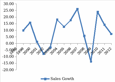
A closer look into the income statement reveals that the growth in net sales has not been that high, though the fall in it too was very prominent. The net sales was found to have 25 percent in 2008 thereafter falling to 6 percent in 2009, then plunging down to a negative 20 percent in 2009. However, in 2010 it rose back by 30 percent falling back in 2011 to 8 percent but slightly increasing in 2012 to 9 percent. This discrepancy in the growth of net sales and sales growth demonstrates that the operating cost or expenses of the company too have been fluctuating at an inconsistent rate.
Table 1: Correlation Matrix showing the relation in growth rates of sales and operating expenses
Table 1 (shown above demonstrates that the cost of sales has a strong relation with growth of net sales as the correlation found between them is 0.91 indicating that the changes in the growth of cost of sales has been consistent with the changes observed for net sales. However, the relation between growth of net sales and that of research and development expenses is not found to be strong, though it shows a positive relation. This implies that the changes in R&D expenses have been changing in the same direction as the changes in net sales but the intensity of the change has not been very strong. Again, the selling and general expenses show a strong positive correlation with growth of net sales. The income statement of the company from 1998 to 2012 shows a distinctive change towards higher sales figures. However, once cannot be sure if the sales figures demonstrated in the statement are free of any credit receivable during the period. In other words, this figure does not clearly demonstrate if the sales figures shown are free of any future payments that are pending and the firm has not collected it. As we have seen in the policy statement in the annual report of Schneider electrics, any pending payment is not seen to have overcome from the previous sales. Therefore, the firm has to improve its collection process from the market in order to manage the losses it faces due to the lack of process in place to ensure speedy recovery/collection from the market.
Analysis of Historical Balance Sheet (consolidated)
The analysis of the consolidated balance sheet from 1998 to 2012 demonstrates quite a lot about the company’s financial health over the period of fourteen years. The balance sheet provides a proper glimpse into the cash flow and the accounts receivable and payable of the company. For our analysis, we need to understand the amount of money that is pending in the market that the company is yet to collect. From the consolidated balance sheet estimates, it was clear that the company’s accounts receivable has been quite high. Further, over the years, this has been increasing at a higher rate than the growth rate of sales, indicating that more sales were made at discounted prices or in instalments in order to increase sales. Further, the company is aware of the dangers into entering into a relationship wherein a large sum of money will be receivable in future after the sale is made. In such a case, the counterparties are selected very carefully in order to avoid the risk of loss on trade accounts receivables. Further, in 2011 and 2012 it was observed that there has been an increase in accounts receivables by €230 million in 2011 and €127 million. This increased the working capital requirement for the company, exerting more pressure on the business. The net accounts receivables from trade in 2012 have been estimated to €5289 and in 2011, it was €5402. Accounts receivable for 2011-12 financial year was €4291 million and in 2010-11 period was €4364 million. Receivables due for over a month have been at €395 million in 2012. In addition, receivables due for over four month’s period are €252. Any receivables due for over a period of one year are foregone and are written off from the balance sheet. The impact the accounts receivables has on the equity of the company has been higher in 2012 than in 2011 (Schneider Electrics 2012).
Why do we see the need to do a DSO analysis
An analysis into the accounts receivables of the company for 2012 and 2011 showed that it increased over the years. Accounts receivables show the amount of credit that is pending in market for the goods that are shown sold in the income statement. In other words, the amount of money that is yet to be collected from the market for goods that has already been sold.
Schneider Electrics’ policies show that once the receivables became doubtful, they were left, and were not collected from the market. The doubtful accounts were first identified, and then they were written off from the income statement. The process of identifying a doubtful account is based on calculating the age of the receivables and then a detailed assessment of the credit risks associated with the receivable. Further, the accounts receivables that are found to be due over a year are discounted.
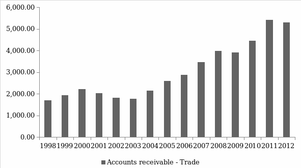
Figure one shows that the accounts receivables for Schneider electrics have been increasing constantly. Therefore, the increasing trend of accounts receivable actually shows that the company’s credit sales have been increasing over the years.
DSO analysis is the first step towards understanding the efficiency of the firm. As it helps us to understand the number of days on e an average a firm takes to recover its pending payments on sales already made, it is an important indicator into the money recovery policy of the firm. In case of Schneider electrics, it is states as a policy by the company that any receivable older than one year were foregone. Nevertheless, the amount of receivable that is pending in the market for the company within a one-year period is more than three thousand million euro. This too is a large amount consistently ranging from 20 to 25 percent of the total sales. In other words, 20 to 24 percent of the total sales of Schneider Electrics have been amount of money that was receivable within the period of 1998 to 2012. The next section will demonstrate the way we have calculated the DSO of the firm over the period of 1998 through 2012.
DSO
The first step in understanding the efficiency of the company is taking DSO level of the company and benchmarking it to the industry or national level. This allows the company to understand if their policy of giving credit and sales credit to end customers is efficient or not. Traditionally, accounts receivables are observed as the measure that is to be targeted to move faster in order to drive down DSO. However, companies are not always successful in creating a seamless order to cash cycle that would help them to minimize DSO. This section will show how DSO has been calculated for the purpose of the present case study and how DSO has altered historically for Schneider Electrics.
Calculation of DSO
Traditionally the formula used for the calculation of DSO as mentioned earlier in the paper is total number of days divided by accounts receivable turnover. In our study as we used annual data therefore the number of days is taken to be 365. Accounts receivable turnover is the ratio of sales to accounts receivables of the company for that period. Here we derived the sales figures from the income statement of the company and the trade accounts receivable data from the balance sheet.
An example of the calculation is presented below for the year 2012. In 2012, the sales of Schneider Electrics is €23946 (all data in millions). The accounts receivable for trade is €5289. To calculate accounts receivable turnover we divide the sales by accounts receivable for trade i.e. 23946 / 5289 which gives us 4.53. This figure is then used to divide the number of days in the period. In case of this analysis, we have taken annual data therefore the number of days in the period being 365. Therefore, in order to get the average payment days of DSO we divide 365 by 4.53. This gives us the figure 80.6. Intuitively, it can be said that 80.6 days is the average collection period for the company in 2012 for collecting the receivables. In other words, the number of days it took the company to turn order to cash in 2012 was 80.6 days.
Historical DSO trend
The DSO calculated for Schneider Electrics over the period of 1998 to 2012 is shown in the following figure. It shows that the DSO of Schneider Electrics has changed over time. The line graph demonstrating the historical movement of DSO shows that it has fallen and then again risen over the years. In recent time, DSO was found to have reached a maximum of 90.6 days in 2009. Then again fallen back to its average level of 82 in 2010 and 2011 again falling partially to 80.6 in 2012.
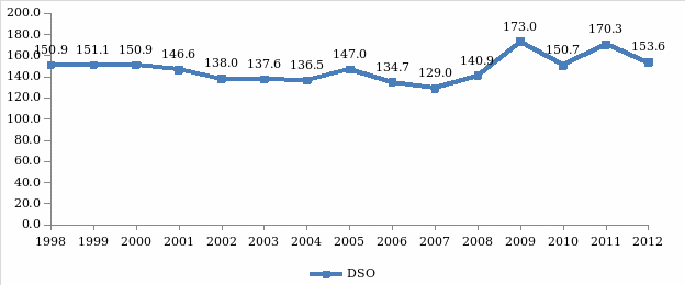
Benchmarking DSO
This section will benchmark the DSO of Schneider Electrics with that of the energy industry (data derived from gurufocus.com (2013)). The data demonstrates that the DSO of the company did not follow the trend in the industry DSO. Table 2 below shows that descriptive statistics of the annual DSOs from 1998 through 2012. It shows that the average of the DSOs for the 15 year period has been almost similar for both the industry and the company. However, the sample variance has been found to be very high. That is why a further analysis into the difference and similarities between the DSO of the two is important.
Table 2: Descriptive Statistics (DSO of Energy Industry and Schneider Electrics)
We conduct a one-factor ANOVA test on the DSO values for Schneider Electrics and the energy industry DSO data. The data (shown in table 2) demonstrates that the F value is 0.02 higher than the F critical value, which is 4.2 indicating that the performance of Schneider Electric’s is not better than the industry. However, the analysis is not statistically significant.
Table 3: ANOVA analysis of DSO of Schneider Electrics and the Industry
Profit Margin
Profit margin is an indicator of the profitability of a company. This demonstrates how a company has been faring in terms of the profits it has earned over the years. Figure 4 demonstrates the historical calculation of the profit margin (net) data of Schneider Electrics from 1998 to 2012.
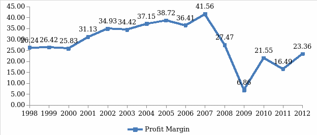
This shows that the profit margin of the company has been declining since 2009 and it had gone back to a level of 39 as was the case in 1998. Therefore, the profitability of the company has shown a fall of 7 percent in 2012 and 11 percent in 2010.
Hypothesis
From the above research and study, we develop two hypotheses for testing in this paper.
- Hypothesis 1: DSO, DSI, DPO, and CCC are negatively associated with profit margin.
The rationale for this hypothesis lies in the fact that higher the DSO, higher is the number of days taken by the firm in collecting its receivable cash outstanding in the market. A higher DSO would have a higher impact on the liabilities of the company, thereby, reducing the cash flow in the firm. This intuitively should have a negative impact on the profit margin of the company as it indicates the profitability of the company. The hypothesis stems from the traditional belief and empirical research that increasing working capital would affect profitability negatively (Uyar 2009).
- Hypothesis 2: DSO, DSI, DPO, and CCC have an impact on profit margin.
Days sales outstanding is believed to have an impact on the profitability of the company as it shows the number of days that the company would take to recover its receivable credit. This measure allows us to ascertain how quickly a firm can recover its credit from the market.
Model Development
The model that is adopted for the study is the one presented by Uyar (2009). Uyar studied the effect cash cycle conversion had on the profitability of the firms using ANOVA and correlation analysis. Uyar found a significant negative relation between CCC and the profitability of the company. The hypothesis is tested using regression and correlation analysis. The variables that are used to study the effect on profitability are DSI, DSO, DPO and CCC. Here CCC is the additive summation of DSI, DSO, and DPO. Here the dependent variables used for the study are CCC, DPO, DSO, and DSI. The regression analysis would give us an equation like this:
Profit margin =![]() +β1 DSI + β2 DSO – β3DPO+
+β1 DSI + β2 DSO – β3DPO+![]()
Table 4: Variable and Measures
| Variables | Measures |
| Day Sales Inventory (DSI) | 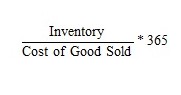 |
| Day Sales Outstanding (DSO) | 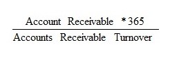 |
| Days Payable Outstanding (DPO) | 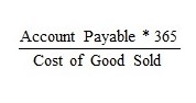 |
| Cash conversion cycle (CCC) | CCC= DSI +DSO-DPO |
| Profit margin (PM) | 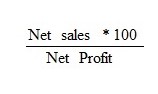 |
The research model therefore may be represented in a diagrammatic form as
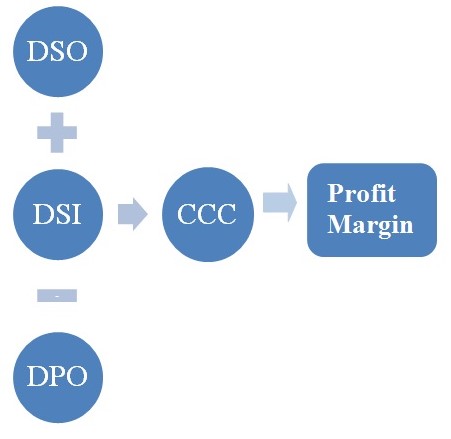
Table 5: Descriptive Statistics of the Variables
Table 5 presents the descriptive statistics that are used for the analysis. The descriptive statistics shows that the mean of the CCC is 169 days. The DPO is less than DSO indicating that the sample of historical data from Schneider Electrics takes more time to collect its bills (147 days) than to pay their bills (96 days).
We conducted a correlation analysis to identify the relationship between the CCC and profitability (PM). The results are shown in the following table.
Table 6: Pearson’s Correlation of the variables
Table 6 demonstrates that the correlation between profit margin and CCC is negative relation with profit margin as has been observed in previous empirical researches. In case of Schneider Electrics, it was found that over the years, cash cycle conversion had a negative relation to the profit margin earned by the company. This throws serious implications to the mangers of the company regarding the importance of managing cash cycles properly for higher the cash cycle great is the negative impact on profitability of the company.
In order to further verify the findings of the data, we conduct a regression analysis of the historical data collected from Schneider Electrics financials. As this analysis gives an inconsistent result for DSO we conduct another multivariate regression of profit margin using DSO as the independent variable.
Table 7: Regression analysis of Profit margin with DSO, DPO, and DSI as the independent variable
Table 7 demonstrates the regression analysis of profit margin with DSO as the independent variable. The analysis shows that the coefficient of DSO is negative (-0.41) and the value is statistically significant at 99 percent level. Therefore, there is 99 percent probability of the regression being statistically significant in its results and it has 99 percent chance of being true. Overall, the regression demonstrates that the model has a 84 percent of the observed variability of DSO as the value of R square is 0.84. This can be explained by the differences in the independent variable. Further negative beta coefficients of the variables are DPO (-.26) and DSO (-.41) which means that an increase of these variables brings about decrease in profitability. At the same time, positive beta coefficient of the variables DSI (.00) means that an increase of these variables brings about increase in profitability.
Intuitively, it can be concluded from the regression results that Schneider Electrics over the years has faced a high DSO and has overlooked the negative correlation between its DSO, DPO and profitability. As it had been seen earlier, average DSO was higher than average DPO implying, payments were made before sale payments were received. Moreover, the gap in average DPO and DSO was very high. Thus, it must be noted that the company over the years has faced a high cash cycle, which has negatively affected its profitability.
Hypothesis Testing
The paper developed two hypotheses that are analysed in the following section.
- Hypothesis 1: DSO is negatively associated with profit margin.
From the regression analysis, it can be said that DSO has a negative effect on the profit margin of the company. The beta coefficient for DSO in the above regression is -0.41 and the p value is 0.00 (<0.05). Therefore, we may accept the hypothesis.
- Hypothesis 2: DSO has an impact on profit margin.
The DSO has a moderate impact on the profit margin of the company. This is found to be true due to the high value of r square of the regression at a statistically significant level. The regression has 99 percent chance of being true, thereby making it highly likely. Thus, we may accept the second hypothesis too that DSO has a strong influence on profit margin.
Past and Present Level of DSO and Profit Margin
Table 8: Historic level of DSO and Profit margin
Table 8 presents the past and the present level of profit margin and the DSO of the company. It demonstrates that the profit margin of the company has been increasing while the DSO has been declining and vice versa. The total average profit margin of the company over the period of 15 years is 28.57 percent and the average DSO for 15 years is 147 days. Graphically the inverse relation between the two is evident. This may further be analysed using statistical tools.
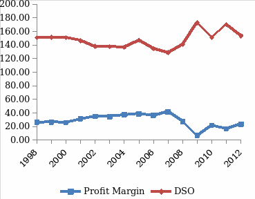
Impact of DSO and Profit Margin on working capital
The working capital or the maturing liabilities of the company can be determined by the amount of assets that can be quickly transformed into cash and the liabilities that has to be settled with twelve months period respectively. Weygandt (2006) points out that a longer DSO results in lower cash being available to the firm for meeting maturing obligations. Therefore, the cash ratio and DSO are expected to have a negative relation.
Table 9: impact of Profit margin and DSO on Cash Ratio
Table 9 demonstrates that the DSO has a negative relation with the Cash ratio of the company. Over the years a negative relationship has been established between cash ratio i.e. the maturing cash requirements of the company in form of current assets and liabilities and DSO. The present regression supports the findings by Weygandt (2006) indicating that the company has had a negative impact on catering to its immediate cash needs due to high DSO i.e. average collection days. The relation between cash ratio and DSO establishes the fact the great is the number of days required in collecting the receivables from the market, the working capital and the availability of cash would be negatively affected. On the other hand, profit margin is found to have a positive effect on cash ratio as it shows that as the company gains greater profit it will have a higher positive impact on cash ratio i.e. the availability of cash to the firm.
Optimal Level of DSO and Profit Margin
Profit margin of Schneider Electrics has been increasing over the years with partial changes. The DSO however, has mostly increased over the years. According to literature both, these have a strong impact on the cost structure of the company. This section tries to find the optimal amount of DSO and profit margin that would not increase operating costs further up. Stickney and Weil (2008) defines profit margin is the percentage of profit realizable from a unit of sale. He states several categories of margins including gross, operating, and net margins. For this analysis, we have taken net profit margin and DSO as the independent variables and analyse their effect on operating expense margin. Operating expense margin is the operating expense that the company has to undertake to continue its operations as a percentage of sales. A regression analysis demonstrates that the DSO has a positive relation (beta coefficient being.01) with operating cost margin indicating that the higher the DSO greater will be the cost and the profit margin is found to have a negative relation with the independent variable (its beta coefficient being -.01). Operating margin is derived from deducting operational cost from the gross margin. Net margin is derived from deducting total costs from revenue and expressing it as a percentage of sales. According to Stickney and Weil (131), a high level of profit margin increases the company’s ability to make profits. However, it also means setting higher prices for customers thus potentially reducing total sales. Since the overall profitability is determined by the price and amount sold, any policy that increases prices is likely to affect the amount of sales from customers. Therefore, setting the profit margin is also a balancing act that entails increased prices to a point that it will not affect the sales of the company.
Weston (2010) offers that the price set for a particular product depends on a number of factors. For an international company as Schneider Electric, the prices depend on competition, cost of production, liable cost, location, taxes among other factors. This means that the company cannot arbitrarily set its profit margin without regard to these additional factors. Weston also offers that profit margin is a good indicator of the cost structure of the company for the period under review. According to Ehrhardt and Brigham (2010), if the profit margin for company is rising, it means that the operational costs for the company are increasing. On the other hand, if the profit margin is falling, it indicates that the operational costs for the company are increasing. Therefore, the profit margin is a good indicator of the cost structure of the company and indicates the management ability to maintain costs at a manageable level. Ehrhardt and Brigham (2010) also cite that a falling profit margin is a management indicator for the need to streamline firm’s operations to reflect the rising cost structure against falling revenues.
Following the optimality rule in economics, we know that profit is optimal when marginal cost equals marginal revenue. In this case, the marginal cost is the operating expense margin and the marginal revenue is the net sales margin. When these equal each other, we will get the optimal amount of profit.
Table 10: Optimality of profit margin
A regression analysis of profit margin as the dependent variable and gross margin and operating margins as the independent variables as pointed out by previous studies (Weston 2010; Ehrhardt & Brigham 2008). The regression overall presents statistically significant F value at 0.0001 (<.05). The R square is found to be.69 indicating 69 percent chance of the results to reoccur. The regression equation formed from the analysis is as follow:
Profit margin = -692.29 + 711.37 gross margin + 767.72 Operating margin
The beta coefficients of gross and operating margin are found to be statistically significant with p-value less than.05. An optimal profit margin may be derived when both gross and operating margin are at its maximum i.e. 1. Therefore, the optimal profit margin according to this equation is 786.8.
The optimality test for DSO is derived by taking it to be the dependent variable and the independent variables as working capital ratio and current ratio. Working capital ratio is calculated as the ratio of sales to the summation of accounts receivable, inventories minus accounts payable. The current ratio is a ratio of current assets to current liabilities.
Table 11: Regression analysis of DSO as dependent variable
The equation derived from the equation is as follows:
DSO = 119.36 + 29.23 Working capital ratio +23.29 current ratio
As we have learnt from the previous literature on DSO that the lesser the DSO it is better for the profitability of the company. However, if DSO is zero then it will mean that the company had to forego many sale opportunity due to its conservative credit policies. Therefore, an optimal level of DSO will help the company attain the maximum possible profit. For this, we must assert the amount of working capital requirement and the ratio at which it has the capability of converting its current assets to current liability. However, we have to find the optimal DSO by minimizing the number days required for cash cycle conversion. In this respect, the lowest value of working capital ratio and current ratio can be zero as both have a positive effect on DSO. Therefore, the optimal level of DSO of derived from this regression analysis is 119.36.
Data Analysis of 4 companiesHistorical DSO and Profit Margin
The companies that are taken for the analysis are Schneider Electrics, General Electric, ABB, and Siemens. These companies operate in the same energy market as Schneider and are competitors.
Table 12: Historic DSO and Profit margin for the 4 companies
Table 10 demonstrates that the average range of DSO is highest for GE (General Electric) and minimum for Siemens. The average DSO for GE is 760 days, which is very high. That of Siemens is just 80 days. This implies that the number of days taken by GE to collect its receivables is almost two years, which is a very long cycle. The average DSO for ABB is 169 days and that of Schneider is 90 days.
Table 13: Descriptive Statistics of the data
Table 11 presents a descriptive statistics of the different variables used for the analysis. The average mean DSO is found to be higher than the DPO, which indicates that the companies in the energy sector tend to clear off their payables before they receive cash from their receivables. This indicates that the companies would face a cash crunch as they have to pay off much before they usually expects return cash from their sales. The CCC for the companies is high at 216 days, which is much higher than the industry standard.
Effect of DSO on Profit Margin
Table 14: Correlation Analysis of the variables
Table 12 demonstrates a correlation analysis of the five variables. From the analysis it can be distinctly observed that day sales inventory has a negative relation to Profit margin, while the other variables such as DSO, DPO, and CCC have a positive impact on profit margin. This finding is different from the previous research findings as discussed in the literature review. For most of the prior empirical researches established that DSO has a negative effect on the profitability of the company. Similar results have been found even in case of analysis of the historic data from the financials of only Schneider Electrics. We may assume that the discrepancy in the findings in case of the data for the four companies may be due to the high DSO calculated for GE and ABB, which have affected the correlation results. Further, the high DSO and the other measures of GE have created a high degree of variation in the data that may have contributed to the deviant result.
Doing a regression analysis of DSO and profit margin, we get the following result.
Table 15: Regression analysis of profit margin and DSO
The regression results are inconclusive, as they do not present any statistically significant result for the study. Further, this too shows a positive beta coefficient for DSO which indicates that for this sample the DSO is positively related to profitability. However, this result is not statistically significant at 95 percent significance level. Further, the R square demonstrates that it has only 11 percent chance of being true limiting the scope for generalizing the findings of the regression analysis.
Impact of DSO and Profit margin on immediate cash requirement
This analysis is done simply by finding a correlation between the cash ratio and DSO and profit margin. Cash ratio is the ratio of cash and cash equivalents to current liabilities. The regression analyses done on cash ratio as the dependent variable and DSO and profit margin as independent variables are presented in table 14. Clearly, the regression analysis shows that the correlation between cash ratio and DSO is negative but it has a positive relation with profit margin. Intuitively it can be stated that the cash ratio is the measure of the company’s liquidity. Nevertheless, higher the DSO, i.e. greater the number of days to collect the receivables, lower would be liquidity. As the company takes longer time to collect its receivables, the cash availability with the company will be lower thereby reducing its liquidity and working capital. It will have less cash to deal with its immediate liquidity requirements. However, higher the profitability i.e. higher the profit margin of the company greater would be its liquidity. The beta coefficient of the DSO is -.00013 is statistically significant (p-value =.00024 <0.05) and that of profit margin is.04 but this result is not statistically significant with p-value (0.06) greater than 0.05. The overall result of the regression is found to be statistically significant with the F value (.0002) being less than.05. The R square value is.79 indicating a 79 percent chance of the regression results repeating it.
Table 16: Regression analysis of cash ration vis-a-vis DSO and profit margin
Optimal level of DSO and Profit margin
In order to find the optimal level of profit margin it must be observed in the data at what point the profit margin is maximum and at what point DSO is least.
Table 17: optimal level of profit margin
Table 15 presents the regression that would enable us to form an equation to determine the optimal level of profit margin. Stickney and Weil (2008) a high level of profit margin increases the company’s ability to make profits. However, it also means setting higher prices for customers thus potentially reducing total sales. Therefore, in order to gain higher profit the firms will end up charging a premium price, which would reduce sales as higher prices, would reduce demand assuming normally elastic law of demand. Hence it is imperative that the firms find an optimal level of profit margin. In order to find it we use two other ratios operating margin and gross margin as out independent variable. The reason for using these variables as our independent variable is operating margin helps us get the amount of variable cost associated with the production and therefore it provides the profit that we will receive due to it and gross margin provides the profit that is earned solely by the sale of goods, keeping all other expenses at bay. Since the overall profitability is determined by the price and amount sold, any policy that increases prices is likely to affect the amount of sales from customers. Therefore, setting the profit margin is also a balancing act that entails increased prices to a point that it will not affect the sales of the company.
A regression analysis is conducted with profit margin as the dependent variable and gross and operating margin as the independent variables. This shows that greater the gross margin i.e. the profit gained just by deducting cost of sales from the total revenue is positively related to the profit margin. The beta coefficient for gross margin is 9.27 with a p-value of.03 (<0.05). the beta coefficient of operating margin is -1.5 with p-value of.07 (>.05). Thus, we see that the beta value of gross margin is statistically significant whereas that of operating margin is not. Overall, the regression analysis gives an R square value of.45 indicating a 45% chance of the occurrence of the results. The over F value (.04) is found to be significant at 95 percent significance level.
Weston (2010) offers that the price set for a particular product depends on a number of factors. For an international company as Schneider Electric, the prices depend on competition, cost of production, liable cost, location, taxes among other factors. This means that the company cannot arbitrarily set its profit margin without regard to these additional factors. Weston also offers that profit margin is a good indicator of the cost structure of the company for the period under review. According to Ehrhardt and Brigham (2008), if the profit margin for company is rising, it means that the operational costs for the company are increasing. On the other hand, if the profit margin is falling, it indicates that the operational costs for the company are increasing. Therefore, the profit margin is a good indicator of the cost structure of the company and indicates the management ability to maintain costs at a manageable level. Ehrhardt and Brigham (58) also cite that a falling profit margin is a management indicator for the need to streamline firm’s operations to reflect the rising cost structure against falling revenues. The regression analysis is supported by the findings of previous researches by Ehrhardt and Brigham (2010) and Weston (2010) both of whom support the fact that an increase in operating cost would lead to an increase in profit margin. The profit margin is positively affected with an increase in the variable cost as there is a greater production, thus greater sales and hence greater profit. The regression equation derived from the analysis is as follows:
Profit margin = 5.05 – 1.5 Operating margin + 9.27 Gross margin
In the above equation, for profit margin to become optimal, it is necessary for operating margin to be zero, thus diluting the negative effect of the operational costs. Further, as the maximum gross margin that we may derive is 1, therefore taking gross margin to be 1 we may calculate the maximum profit margin which is 14.32 percent.
Conclusion
The analysis of DSO and profit margin for Schneider Electrics using annual financial data from the company demonstrated that the DSO and profit margin have a strong negative relation. The literature review will now present the current research into the three research questions set for the study. The literature review for this research project will be centred on the research question set at the beginning. The research analysis of DSO and profit margin for Schneider electrics and the four major companies in the energy management industry are analysed in the paper. The analysis was done in the form of a case study in which we first tried to understand the background, strengths, weaknesses, and opportunities for Schneider Electrics. In the conclusion of the paper, we summarise the findings of the overall research based on the two distinctions used for the analysis. The first will deal with the research findings of annualised financial data of Schneider Electrics and the second will be the financial data analysis of four companies operating in energy management industry.
Overall, the DSO of the company has been found to be lower than the industry level of DSO, which indicated that overall, the DSO was better off and the company took care to control the accounts receivables. Further, the cases study demonstrated that the company wrote-off all receivables that were older than one year. This policy led to further problems in its relation to the profitability of the firm. The two other variables that the research analysed were DPO and DSI. Overall, the regression analysis of DSO as the independent variable and profit margin as the dependent variable indicated that the DSO has a statistically significant negative influence on profit margin. Further negative beta coefficients of the variables are DPO (-.26) and DSO (-.41) which means that an increase of these variables brings about decrease in profitability. At the same time, positive beta coefficient of the variables DSI (.00) means that an increase of these variables brings about increase in profitability. Intuitively, it can be concluded from the regression results that Schneider Electrics over the years has faced a high DSO and has overlooked the negative correlation between its DSO, DPO and profitability. As it had been seen earlier, average DSO was higher than average DPO implying, payments were made before sale payments were received. Moreover, the gap in average DPO and DSO was very high. Thus, it must be noted that the company over the years has faced a high cash cycle, which has negatively affected its profitability. The results were found consistent with previous research findings. There has been much research delineating the relation between cash cycle conversion and profitability. Usually businesses sell their product on discount or on terms of instalment payments. Longer the period of these payments, stronger would be the negative effect on working capital of the firm. Faster the payments are made to the firm, easier it would be for the company to manage its working capital and thereby its performance. Stickney and Weil (2008), a high level of profit margin increases the company’s ability to make profits. However, it also means setting higher prices for customers thus potentially reducing total sales. Since the overall profitability is determined by the price and amount sold, any policy that increases prices is likely to affect the amount of sales from customers. The results of the regression analysis shows similar results.
The impact DSO and profit margin had on maturing obligations was tested using regression analysis with cash ratio as dependent variable and DSO and profit margin as the independent ratio. On analysing the data from only Schneider Electrics it was found that the DSO has a negative relation with the Cash ratio of the company. Over the years a negative relationship has been established between cash ratio i.e. the maturing cash requirements of the company in form of current assets and liabilities and DSO. The present regression supports the findings by Weygandt (2006) indicating that the company has had a negative impact on catering to its immediate cash needs due to high DSO i.e. average collection days. The relation between cash ratio and DSO establishes the fact the great is the number of days required in collecting the receivables from the market, the working capital and the availability of cash would be negatively affected. On the other hand, profit margin is found to have a positive effect on cash ratio as it shows that as the company gains greater profit it will have a higher positive impact on cash ratio i.e. the availability of cash to the firm.
Similar results were found for the data analysed from the four competing firms. The analysis showed that the cash ratio is the measure of the company’s liquidity. Nevertheless, higher the DSO, i.e. greater the number of days to collect the receivables, lower would be liquidity. As the company takes longer time to collect its receivables, the cash availability with the company will be lower thereby reducing its liquidity and working capital. It will have less cash to deal with its immediate liquidity requirements. However, higher the profitability i.e. higher the profit margin of the company greater would be its liquidity. The beta coefficient of the DSO is -.00013 is statistically significant (p-value =.00024 <0.05) and that of profit margin is.04 but this result is not statistically significant with p-value (0.06) greater than 0.05. this study too was consistent with the results of the previous researches.
The optimal level of DSO and profit margin are derived from an analysis of the two with respect to their component factors. This too is derived by using regression analysis of both the datasets. Stickney and Weil (2008) a high level of profit margin increases the company’s ability to make profits. However, it also means setting higher prices for customers thus potentially reducing total sales. Therefore, in order to gain higher profit the firms will end up charging a premium price, which would reduce sales as higher prices, would reduce demand assuming normally elastic law of demand. Hence it is imperative that the firms find an optimal level of profit margin. In order to find it we use two other ratios operating margin and gross margin as out independent variable. The reason for using these variables as our independent variable is operating margin helps us get the amount of variable cost associated with the production and therefore it provides the profit that we will receive due to it and gross margin provides the profit that is earned solely by the sale of goods, keeping all other expenses at bay. Since the overall profitability is determined by the price and amount sold, any policy that increases prices is likely to affect the amount of sales from customers. Therefore, setting the profit margin is also a balancing act that entails increased prices to a point that it will not affect the sales of the company.
A regression analysis is conducted with profit margin as the dependent variable and gross and operating margin as the independent variables. This shows that greater the gross margin i.e. the profit gained just by deducting cost of sales from the total revenue is positively related to the profit margin. The beta coefficient for gross margin is 9.27 with a p-value of.03 (<0.05). The beta coefficient of operating margin is -1.5 with p-value of.07 (>.05). Thus, we see that the beta value of gross margin is statistically significant whereas that of operating margin is not. Overall, the regression analysis gives an R square value of.45 indicating a 45% chance of the occurrence of the results. The over F value (.04) is found to be significant at 95 percent significance level. Thus, the research paper successfully answers the three research questions based on which the whole paper has been modelled.
References
Adams, C, Hoque, Z & McNicholas, P 2006, ‘Case Studies and Action Research’, in Z Hoque (ed.), Methodological Issues in Accounting Research: Theories, Methods and Issues, Spiramus Press Ltd., London.
Ahrens, T & Chapman, CS 2006, ‘Doing qualitative Weld research in management accounting: Positioning data to contribute to theory’, Accounting, Organizations and Society, vol 31, no. 8, pp. 819-841.
Bartunek, JM, Rynes, SL & Ireland, RD 2006, ‘What makes management research interesting and why does it matter?’, Academy of Management Journal , vol 49, pp. 9-15.
Benishay, H 1965, ‘Managerial Controls of Accounts Receivable: A Deterministic Approach’, Journal of Accounting Research, vol 3, no. 1, pp. 114-132.
Bennett, A & Elman, C 2006, ‘Qualitative research: Recent developments in case study methods’, Annual Revew of Political Science, vol 9, pp. 455-476.
Capkun, V, Hameri, A-P & Weiss, LA 2009, ‘On the relationship between inventory and financial performance in manufacturing companies’, International Journal of Operations & Production Management, vol 29, no. 8, pp. 789-806.
Carpenter, MD & Miller, JE 1979, ‘A reliable framework for monitoring accounts receivable’, Financial Management , pp. 37-40.
Ching, HY, Novazzi, A & Gerab, F 2011, ‘Relationship between working capital management and profitability in Brazilian listed companies’, Journal of global business and economics, vol 3, no. 1, pp. 74-86.
Christopher, S & Kamalavalli, A 2009, Sensivity of profitabiltiy to working capital management in Indian corporate hospitals, Web.
DeHoratius, N & Rabinovich, E 2011, ‘Field research in operations and supply chain management’, Journal of Operations Management, vol 29, no. 5, pp. 371-375.
Deloof, M 2003, ‘Does working capital management affect profitability of Belgian firms?’, Journal of Business Finance & Accounting , vol 30, no. 3/4, pp. 573-588.
Dorsman, A & Gounopoulos, D 2008, ‘Controlling working capital in multinational enterprises’, Journal of Corporate Treasury Management , vol 2, no. 2, pp. 152-159.
Ebben, JJ & Johnson, AC 2011, ‘Cash Conversion Cycle Management in Small Firms: Relationships with Liquidity, Invested Capital, and Firm Performance’, Journal of Small Business & Entrepreneurship , vol 24, no. 3, pp. 381-396.
Ehrhardt, M & Brigham, E 2008, Corporate Finance: A Focused Approach, John Wiley & Sons, Hoboken, NJ.
Eisenhardt, KM 1989, ‘Makinf Fast Strategyc Decisions in High-Velocity Environemnts’, Academy of Management Journals, vol 14, pp. 532-550.
Eisenhardt, KM & Graebner, ME 2007, ‘Theory Building from Cases: Opportunities adn Challenges’, Academy of Management Journal, vol 50, no. 1, pp. 25-32.
Ek, R & Guerin, S 2011, ‘Is there a right level of working capital?’, Journal of Corporate Treasury Management, vol 4, no. 2, pp. 137-149.
Etiennot, H, Preve, L & Sarria-Allende, V 2012, ‘Working Capital Management: An Exploratory Study.” 22.1 (2012): 161-174.’, Journal of Applied Finance, vol 22, no. 1, pp. 161-174.
Evans, JR 2004, ‘An exploratory study of performance measurement systems and relationships with performance results’, Journal of Operations Management , vol 22, no. 3, pp. 219-232.
Fisher, M 2007, ‘Strengthening the empirical base of operations management’, Manufacturing & Service Operations Management , vol 9, no. 4, pp. 368-382.
Freitas, LP 1973, ‘Monitoring Accounts Receivable’, Management Accounting, vol 55, no. 3, pp. 18-21.
Gallinger, GW & Ifflander, AJ 1986, ‘Monitoring accounts receivable using variance analysis’, Financial Management, vol 15, no. 4, pp. 69-76.
García-Teruel, Juan, P & Martínez-Solano, P 2007, ‘Effects of working capital management on SME profitability’, International Journal of Managerial Finance , vol 3, no. 2, pp. 164-177.
Gilbert, CJG 2005, ‘Unbundling the Structure of Inertia: Resource versus Routine Rigidity’, Academy of Management Journal, vol 48, pp. 741-763.
Gill, A, Biger, N & Mathur, N 2010, ‘The relationship between working capital management and profitability: evidence from The United States’, Business and Economics Journal , vol 10, pp. 1-9.
Granlund, M 2001, ‘Towards explaining stability in and around management accounting systems’, Management Accounting Research , vol 12, no. 2, pp. 141-166.
GuruFocus.com 2013, Energy Industries, Inc. Days Sales Outstanding, Web.
Hofmann, E, Maucher, D, Piesker, S & Richter, P 2011, ‘Determination of the Internal Financing Power of Corporate Growth via the Self-Financeable Growth Rate’, Professional Supply Management , vol 1, pp. 7-12.
Houston, J & Brigham, E 2009, Fundamentals of Financial Management, Southwestern College Publishing, Ohio.
Hutchison, PD, Farris, MT & Anders, SB 2007, ‘Cash-to-cash analysis and management’, CPA Journal, vol 77, no. 8, pp. 42-46.
Inman, RA, Sale, ML & Green, KWJ 2009, ‘Analysis of the relationships among TOC use, TOC outcomes, and organizational performance 29.4 (2009): 341-356.’, International Journal of Operations & Production Management, vol 29, no. 4, pp. 341-356.
Jeffery, C 2007, ‘Working capital: Measurements and techniques for the treasurer’, Journal of Corporate Treasury Management, vol 1, no. 2, pp. 115-119.
Jose, ML, lancaste, C & Stevens, JL 1996, ‘Corporate return and cash conversion cycle’, Journal of Economics and Finance, vol 20, no. 1, pp. 33-46.
Lazaridis, I & Tryfonidis, D 2006, ‘Relationship between working capital management and profitability of listed companies in the Athens stock exchange’, Journal of Finance and Analysis, vol 19, no. 1, pp. 26-35.
Lewellen, WG & Edmister, RO 1973, ‘A general model for accounts receivable analysis and control’, Journal of Financial and Quantitative Analysis, pp. 195-206.
Lewellen, WG & Johnson, RW 1972, ‘Better way to monitor accounts receivable. Graduate School of Business Administration, Harvard University, 1972.’, Harvard Business Review, pp. 101-109.
Mohamad, NEAB & Saad, NBM 2010, ‘Working capital management: The effect of market valuation and profitability in Malaysia.” 5.11 (2010): p140.’, International Journal of Business and Management, vol 5, no. 11, pp. 140-147.
Padachi, K 2006, ‘Trends in working capital management and its impact on firms’ performance: an analysis of Mauritian small manufacturing firms’, International Review of Business Research Papers , vol 2, no. 2, pp. 45-58.
Paul, SY, Devi, SS & Teh, CG 2012, ‘Impact of late payment on Firms’ profitability: Empirical evidence from Malaysia’, Pacific-Basin Finance Journal, vol 20, no. 5, pp. 777-792.
Preve, L & Sarria-Allende, V 2010, Working capital management, Oxford University Press, Oxford, UK.
Reilly, G & Reilly, R 2002, ‘Performance Measurement for Improved Working Capital Management’, Journal of Cost Management , vol 16, pp. 13-20.
Scapens, RW 1990, ‘Researching management accounting practice: the role of case study methods ‘, The British Accounting Review, vol 22, no. 3, pp. 259-281.
Scapens, RW 2006, ‘Understanding management accounting practices: a personal journey’, The British Accounting Review , vol 38, no. 1, pp. 1-30.
Scherr, FC 1989, Modern working capital management: text and cases, Prentice Hall, New Jersey.
Schneider Electrics 2012, Annual Report, Web.
Schneider Electrics 2013, Schneider Electrics, Web.
Shafer, SM & Moeller, SB 2012, ‘The effects of Six Sigma on corporate performance: An empirical investigation’, Journal of Operations Management.
Singhal, K & Singhal, J 2012, ‘Imperatives of the science of operations and supply-chain management ‘, Journal of Operations Management, vol 30, no. 3, pp. 237-244.
Stickney, C & Weil, R 2008, Financial Accounting: An Introduction to Concepts, Methods, and Uses, South-Western College, New York.
Uyar, A 2009, ‘The relationship of cash conversion cycle with firm size and profitability: an empirical investigation in Turkey’, International Research Journal of Finance and Economics, vol 24, no. 2, pp. 186-193.
van Barneveld, W, Heijes, C, Westerman, W & Westerman, W 2013, The control of working capital: a case study on performance measurement, Web.
Viskari, S, Lukkari, E & Kärri, T 2011, ‘State of working capital management research: bibliometric study’, Middle East Finance Econ , vol 14, pp. 99-108.
Wagner, SM, Grosse-Ruyken, PT & Erhun, F 2012, ‘The link between supply chain fit and financial performance of the firm.” 30.4 (2012): 340-353.’, Journal of Operations Management, vol 30, no. 4, pp. 340-353.
Watson, KJ, Blackstone, JH & Gardiner, SC 2007, ‘The evolution of a management philosophy: the theory of constraints’, Journal of Operations Management, vol 25, no. 2, pp. 387-402.
Weick, WF 2007, ‘The Generative Properties of Richness’, Academy of Management Journal, vol 50, pp. 14-19.
Weston, J 2010, Essentials of Managerial Finance, Dryden Press, Hinsdale.
Weygandt, J 2006, Accounting Principles, John Wiley & Sons, Inc., New York.
Wu, Z & Choi, TY 2005, ‘Supplier–supplier relationships in the buyer–supplier triad: Building theories from eight case studies’, Journal of Operations Management , vol 24, no. 1, pp. 27-52.
Yahoo Finance 2013, Yahoo Finance, Web.
Yin, RK 2009, Case Study Research: Design and Methods, Sage, London, UK.
Appendix
Table 18: Historical Income Statement
Table 19: Historical Consolidated Balance Sheet
Table 20: The variables used for the analysis
Table 21: Data for analysis of 4 companies for years 2009-2012