Evolving of World Economic Geography Concept

Abstract

Chapter one of this study seeks to address how the world economic geography concept evolved. Additionally, evidence of a correlation between manufacturing wages and proximity to demand will be analyzed for a specific duration of time, in this case for 23 years. The study utilized trade gravity equations data from 27 sample industries in the year between 1980 and 2003 to measure market access, otherwise referred to as proximity to demand. After the data analysis, 59% (16) of the sampled industries indicate evidence of wage response. To control for variable bias in the data, the study utilized panel data econometrics. The lack of evidence of market access in this study is explained by various variables such as labor regulations, labor relocation, supplier access, and availability of the human resource.

The changing world economic geography of manufacturing

Over the last three decades or so, the world economic geography in the sector of manufacturing industry has undergone evolutional changes; this has been spurred by rapid globalization and technological advances. Despite this, a conglomeration of the manufacturing process at strategic locations continues to be the trend. The interrelation of various variables such as trade costs, proximity to demand, and input prices is central to the conceptualization of agglomeration process theories such as the Seminal contribution theory so far advanced by Krugman (1991b) in the manufacturing sector. Redding and Venables (2004) for instance have found evidence that market potential empirical data between countries can be utilized to inform on income levels discrepancies, or even choice of location by firms as Head and Mayer (2004a) asserts.

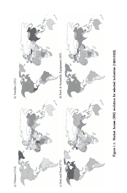
Figure 1 highlights the relationship between demand and production as identified in 4 specific sectors in the manufacturing sector for a given duration (1980-2003). A detailed discussion for this analysis will be provided in a later section (1.4.2), but in general dark shaded countries imply great market access. In summary, the analysis indicates that only two sectors, that of Textile & Iron, and Steel have experienced drastic transformation towards market potential in their countries of operation that is characteristic of redispersion. On the other hand, Professional & Scientific equipment, as well as the Tobacco sector appear less inclined to exhibit patterns of spatial deconcentration which are noticeably dominated by developed countries during the initial stages.

The Economic geography model holds that a correlation exists in the short run between wage and market potential; however, in the long run, a firm’s choice of location is often influenced by low wages among other factors and the resulting industrialization is likely to negatively impact on the market potential thereby causing firm dispersion. This dispersion is further driven by the globalization process because of the way it impacts trade costs. Despite this, dispersion is relatively hard to occur since it is a function of a myriad of other factors such as country profile, level of technology, fiscal policies, labor regulations, and product factors among others; all of which directly impacts market potential and influence its evolution as demonstrated in Figure 1.1.

To investigate the implications of economic geography, various research studies have mainly focused on the concepts espoused on the demand proximity on profits theory which has identified a positive correlation between market access/proximity to demand and the ability of the firm to pay high wages in specific countries. The determination of the positive correlation has been derived from the country-specific GDP per capita regressed across the various countries analyzed. But to strengthen this analysis this study recommends two other strategies; first is that industry heterogeneity should also be assessed when wage levels variable in the industry is used in place of GDP per capita. And secondly, a time dimension should be established so as to help in controlling the effect of heterogeneity in the data. The data in figure 1.1 indicates that the direction of market access is dependent on the type of the sector.

Consequently, in this paper, I seek to investigate the sectors in which the wage variable is most effective in promoting market access evolution. This requires that the data be verified through various tests such as that of robustness across at least two types of market access; the results of this analysis indicate there is a robust coefficient in 16 sectors of the total industries sampled that ranged between 10-37%. When the market access elasticity range is compared with results generated from other similar studies, it is noticeable that the range is on average lower but more close to figures that utilized panel data as has been supported in recent studies by Redding and Venables (2004) and (Mayer, 2008). Additionally, the findings indicate the internal flow variable as a critical component in measuring market access across sectors (Mayer, 2008; Boulhol and de Serres, 2008).

In this study I will also simulate how the wage variable is impacted by two of the most notable international frameworks that facilitate market access through integration; the World Trade Organization (WTO) and the Regional Trade Agreement (RTA). Trade integration frameworks such as these two have positive implications for two types of countries; isolated countries and countries that are geographically located near rich developed countries. Thus, as spatial competition is realigned, countries located at peripherals suffer from decreased market access until demand centers emerge in that region as has been happening in Asia for over the last two decades. In general, there is evidence that a positive correlation exists between market access and manufacturing wages based on the data analysis of the 16 industries, even though the strength of that correlation tends to vary.

This study will be organized in the following way; theoretical framework and analysis of empirical data will be discussed in section 1.2, data and related inferences will be in section 1.3, study simulations will be section 1.4, and finally section 1.5 will conclude the findings of the study.

Theoretical background

In this section, I propose to investigate a competition model that is essentially monopolistic and which exhibits other characteristics such as firm homogeneity, product variety that is experiencing a return on the scale on its costs of trade. Based on this theoretical framework, a “NEG wage equation” can be developed which represents the positive correlation between wage levels and the resulting market access where profit is a zero constant. The implications of this equation imply that firms on average are likely to provide more wages in those countries that are in close proximity to large bustling markets because of the associated low costs in products delivery. In doing this, I relied on the standard procedure outlined by Fujita et al (1999); which gave me the model indicated in the Appendix.

The model disaggregates the economy into two parts based on the nature of trade patterns; the A-sector and the M-sector. In the A-sector of the economy, trade costs are nonexistent, competition is generally perfect and the rate of returns is constant; as such the A-sector is what nurtures spatial specialization because it neutralizes the adverse effect caused by M-sector in the economy. On the other hand, M-sector is characterized by the presence of trade costs of products that exhibit horizontal differentiation; the variables associated with this sector are fi which represents the fixed cost for each plant, and mi, which represents marginal cost constant. Thus, when you apply the formula, a firm’s expected profit in given region i, will be;

π = p_iq_i – m_iq_i – f_i(1.1)

If profit is maximized, a new profit level is achieved as shown

p_i (1.2)

To define profit for a specific regional market j, the demand function as detailed in the appendix is applied as well as the formula for determining gross profit (π_ij = p_ijq_ij/o); thus;π_i =1/σ[p_i^1-σ(Ø_ij]- f_i(1.3)

Further, as described by Baldwin et al (2003), I included the variable “phi-ness” to represent trade liberalization (free-ness) given by Ø_ij Ξ r_ij^1-σ which incorporates two other variables; the elasticity of substitution on demand (O) and the cumulative impact caused by trade costs (τ). The model indicates that the profitability of the trade is dependent on all of these variables since their increase inversely decreases the profitability of the trade as shown except for the variable of local demand (Ø_ij = 0).

Equation wise, an ideal trade process would be depicted by Ø_ij = 1.µY_j which shows costs of M-good incurred by the importer; in this case, the price index (of potential employers) is given by P_j^1-σ as derived in the appendix and is a function of price, trade costs and elasticity of substitution. For this reason, the price index can be used as an indicator of assessing the extent that the market is crowded by the firm considering that increased competition translates to reduced prices, this is what is being termed as a “multilateral resistance term” Baldwin et al (2003).

Thus, in the equation below (1.3) the individual net profits i across regions is the same as total profits in the same region combined, j.

π_i =1/σ– f_i

The function MA on the equation stands for market access/real market potential as defined by Head and Mayer (2004b); MAi is the summation of the market access for every region (i) which is further weighted by the function of accessibility against the same regions, i; Ø_ij is a component of markets j while P_j^1-σ is for the variable of market crowding. From this, we can deduce spatial equilibrium to be determined by hypothesizing that profit is constant for all firms included. By applying the iso-profit equation, we can obtain an equation that relates MA to costs because profit will have been capped at zero as shown below;

MA_i (1.4)

The price version: Market access and factor rewards

In order to arrive at an accurate equation that directly relates together the variables of employment, wages and MA, it is imperative that related factors of production and technology of use, including assumptions made on labor change in the M-sector be factored in. In this case, we shall consider labor to be the only factor of production¹ on the M-sector.

Originally, the A-sector was developed based on the assumption that firm workers are both unskilled and immobile, as represented by u (superscript) while the M-sector firm workers were assumed to have opposite characteristics, mobile and perfect indicated by sk):². Thus,

w_i^skl_i^sk = w_i^sk(a^skq_i + F^sk) (1.5)

So, based on this, firm production is pegged on two types of labor costs; the ask which is only incurred during production and Fsk, which is fixed; both of which applies across regions irrespectively. And as Fijita et al (1999) posits, equation 1.4 will perfectly articulate the variables of an NEG wage equation, since it can be used by a firm to establish the baseline of its wages based on its present or desirable location of business.

(1.6)

Thus far, three of the essential components of an NEG theory have been included and explained; if we include the rest two referred as “endogenous location of demand and endogenous firm locations” NEG will be complete as described by both Baldwin et al (2003) and Fujita et al (1999). In the following section of this paper the rest of these two components of NEG theory will be described and demonstrated as well.

The quantity version: Relocation and the spatial adjustment

If we consider all factors constant similar to general equilibrium, market access on wages is seen to be negatively influenced (reduced) by the presence of labor migration. Thus, if we make a change in the liberalization of trade, say by a reduction in ø_ij impacts on all regions, in the same way, then market access in all those countries will consequently vary from each other. After this to attain previous equilibrium in the same locations will require selective profit equalization; it is this phenomenon that Head and Mayer (2006) attempts to investigate by applying two opposite scenarios that relate to migration; free migration and zero migration.

When zero migration is considered in the equation, the result is increased wages driven by more than average prices of goods, but with free migration, price equalization is attainable. This sparks another chain of events whereby firms again tend to collate in high market access regions due to reduced trade costs; this gradually means the price index P_j^i-σ increases which eventually reduces the overall MA of the region.

In fact, the presence or lack of migration is not the only function that impacts NEG forces and the only one that explains it as Fujita et al. (1999) advances other functions that explain the pattern of costs. This is evident when globalization happens to be the driving force of firms to collate in a given region of strategic importance (core region), after that any more integration is not possible in that region except at the periphery usually through redispersion.

This is well demonstrated by Puga (1999) through the application of input-output linkages as elements of production in firms. Thus, as firm integration continues it spurs intermediates’ growth in the same regions since they are also impacted by trade costs, and more so because input-output linkages slow the agglomeration process that drives the integration. In the meantime, as long as there is the presence of wage gap, firms will continue to agglomerate in countries where the wage is below average in a predictable pattern where such firms will largely constitute those industries that are (1) labor-intensive and (2) involved in producing finished goods that can be shipped to market regions (Zeng, 2006).

The resulting concentration of firms (quantity) in a given region can be determined by focusing on the nature of the agglomeration process as we have just seen. By using this principle Head and Mayer (2006) utilize both wage and unemployment data of firms in collated regions to verify which is more reliable, considering that level of employment in such firms is a direct indicator. Thus, in the empirical section of this paper, this study will apply similar techniques in controlling against the effect of quantity and in the verification of procedures used in analyzing the data.

Identification issues

The impact that economic geography has on the resulting labor trend in a given region is the single most relevant factor that describes the process of industry evolution for the last few decades but is not the only one that influences this evolution. All the same, various research studies notably by Krugman and Venables (1995) however disqualify relying on factors such as endowments and technology change to explain the phenomena of industry evolution primarily because they can be controlled. Similarly, the data used for this study will control the variables such as endowments, technological levels among others in a similar manner. Additionally, GMM (dynamic panel data estimate) analysis that evaluates the relationship between market access and wages is undertaken to establish if this is still the case in most industries. The accuracy of these results is maintained through the use of time-sensitive regression tests that are also widely and effectively used in other models as well.

The GMM analysis of estimation is nevertheless used notwithstanding the challenges posed by it since it is a new model that is still being validated. But this estimation equation is a culmination of relentless effort to establish a working framework that can reliably be used to develop a model of factor proportion that departs from technological evolution theories. A recent study by Fitzgerald and Hallak (2004) is among the few that have effectively managed to modify the Rybczynski equation to develop a model that can be applied in testing technological differentials. But which the authors lament its limitations since “any model that links specialization to the level of development will predict such an empirical relationship” (p. 279) unless endowment factors are no longer linked to the level of development during the accumulation process (Fitzgerald and Hallak, 2004).

Similarly, a study by Romalis (2004) attempts to derive trade patterns based on the variable of factor endowment and economic geography theory and their nature of relationships; in this case, as well, it is impossible to integrate the variables that technology variation and factor accumulation will have in the model. More evidence as presented by Antweiler and Trefler (2002) regarding the phenomenon of “increasing return in world trade” indicates that empirical data is limited in distinguishing between dynamic nature and scale of technology occurring across countries primarily because the change in technology is often driven by dominating large firms. It is therefore clear why formulation of a single model that integrates all these variables is, to say the least, a challenging task, more so when the impacts of such variables require to be individually ascertained.

In general, the models outlined in this study and the resulting findings will indicate a positive correlation between the geographic location of a country and labor outcome, even though this cannot be established by some other estimation techniques. Thus, researchers should keep this in mind and strive to control the results of the resulting association between the above variables with other verifiable techniques under stringent conditions. A recent study by Hering and Poncet (2009) is a valuable resource that can help researchers chart the way forward on this challenging issue as well as the techniques discussed in other Chapters of this paper.

Empirical issues and data

Trade, gravity and economic geography variables

In this model, the price index given by P_j^i-σ is the most tricky when working towards developing a reliable equation; to overcome this challenge I rely on the procedure developed by Redding and venables (2004) which reccomends that the price indexes be linked to the trade gravity equation by way of fixed effect for each country. Besides this, the study suggests that the ø_ij estimate be ensured is accurate as possible because of the relevance that it has in the model as a proxy and its usefulness in capturing a variety of other variables. Additionally, in order to strengthen the accuracy of policy simulations, the authors propose that variables of trade policy be incorporated when working with trade costs. Since the theoretical model developed for this study attempts to investigate the nature of resulting spatial interactions caused by trade, the use of gravity-based regression for purposes of estimation will be very fitting since data of economics involved will be utilized.

Thus, from this analysis, T_ij denote the direction of bilateral export movement originating from i towards j³; by use of the equation in 1.118 the following can be derived.

T_ij = n_ip_ijq_ij =ø_ij(1.7)

In this case, both FMj and FXi which represent importer and exporter fixed effect respectively can effectively be relied upon to integrate all variables that relate to specific regions. The ø_ij which is the phi-ness of trade is a function of 3 categories of variable that can either dissuade or facilitate trade, and include;

1. First category of variables that are considered fixed timewise for instance contiguity Cij ,historical colonial ties Colij, language factor Lij and bilateral distance⁴ dij among others.
2. Category two, variables not fixed in time, mainly trade policy variables of WTOij and RTAij; in this case the effect of these two variables are controlled by using 1 as a dummy where any of the partner country is a signatory to one or both of these trade policies.
3. Category three, a unique dummy variable Bij that controls against the effects of national borders as we shall see in the following section.

Based on these we get;

ln T_ij = FX_i + FM_i + δ ln d_ij + λ₁C_ij + λ₂L_ij + λ₃Col_ij + λ₄RTA_ij,t + λ₅WTO_ij,t + λ₆B_ij + λ₁µ_ij (1.8) From this we can derive ø_ij through the following equation

_Øij = d^δ_ii exp (λ₁Cij +λ₂L_ij +λ₃Col_ij +λ₄RTA_ij,t +λ₅WTO_ij,_t +λ₆B_ij) (1.9)

Since the market potential of a given country is a function of two related components of market access; DMA (domestic market access) and FMA (foreign market access) FMA we can obtain both;

DMA_i = exp (FM_j) d^δ_{ii ;} d^δ_ii =2/3

(1.10)

Here, I end up with two results of market variations that are not consistent because of the inclusion of the Bij variable, which is the national border effect. In the first instance, I utilize a procedure that factors in bilateral elements in overall trade costs without considering the impact of any border effect; as such Bij is set at zero (Redding and Venables, 2004). Because this approach requires use of data generated from bilateral trade between partners, it exempts the rest of the variables that do not apply in international bilateral trade. This however doesn’t limit the study in estimating the country’s national component (normally obtained through use of data generated internally) as this can still be inferred from internal distance and from the associated fixed effect. But, no doubt without using the variable of border effect the study is significantly likely to suffer from bias particularly on the ø_ij element; because of this danger, this study seeks to compartmelize the risk of bias by tagging market access models developed this way as RV method.

The second method advanced by Head and Mayer (2006) suggests that the Bij variable of the border effect be treated differently in domestic trade and international trade, set at 0 and 1 respectively. In using this approach the authors suggest that a proxy of the country and trade be set up where the RV model is applied. Additionally, it is described as necessary to align estimation model to reflect “production minus total exports”; since exportation of a product attracts additional costs, the coefficient for the above variable can only be negative (Head and Mayer, 2006). In determonation of the Tii, variable the study utilized the industrial production figures despite the challenges associated with its availability as detailed in section 1.3.3. So thus far, we obtain our second market access model which will be denoted as HM method.

On equation 1.8, the OLS fixed effects on exporter and importer are used as the basis for estimatimating the industry and the year independently; the use of this estimation in this equation was preferred notwithstanding concerns higligted by other studies regarding the suitability of this estimation approach, in this case I will only higlight two. Foremost, is that estimation equations that are non-linear are highly regarded when the purpose is to analyze trade data; OLS is neither linear nor is it reliable since it generates an uij error that possibly indicates bias when heteroskedasticity occurs. Besides, OLS is limited in the way it manages trade data that has zero values which unfortunately is not only a limitation that is specific to this method but virtually all similar techniques since an effective approach is yet to be developed as many studies laments (Silva and Tenreyro, 2006; Martinez-Zarzoso et al., 2007; Martin and Pham, 2008; Helpman et al., 2008; Silva and Tenreyro, 2009). This is even more elusive when datasets that has significantly high zeroes as is typical of trade data are runned by non-linear method (Buch et al., 2006).

In fact, this was evident in this study when regression of trade data were done at industrial level; the generated zeroes in this case constituted a significant amount of all values which cannot be managed even with Gamma or Poisson method when applied repetitively. To cut down on the zeros generated by the dataset and facilitate nonlinear estimation techniques I used the number of trade partners per country as the criteria of inclusion and exclusion; this way as much as half of the generated zeros were reduced in the final results because only sample countries that had excess of 20 partners were included in the analysis. Because of this, consolidation of the majority of the possible 648 (24 years* 27 industries) regressions is made possible; but unfortunately the validity and quality of some of the resulting analysis are compromised due to inconclusive data used generating fixed effect and border effects.

The second issue is articulately addressed by Baier and Bergstrand (2007) in which they asserts that RTAs and related variables have selection bias that stems from its endogenicity, which can therefore not be controlled through cross-section method of data management. Because the interest of this study is to generate coefficients that relate to specific years, I disregard the use of panel data method that is suggested by Baier and Bergstrand (2007) in light of cross-section method limitations. In any case given the nature of “downward bias” that is described to occur in cross-section, the implications is that any bias occurring in market access as a result of this will not have adverse implications on the results since such bias is essentially lower-bound and would therefore not be a concern to this study theoretically or practically. In the following section this paper will focus on NEG wage equation and related tests.

Panel estimation of the NEG wage equation

By using equation 1.6 which is a log-linear estimation, we can derive a relationship regional wage and MA variable as indicated below

ln w_i = ς₁ +σ^-1 ln MA_i, +ìX_i + v_i (1.12)

In this case, wi stands for wage variable (w) for a specific region (i), since only data pooled from manufacturing industries are utilized here, sk does not apply.

Using this equation the MA coefficient is the same as the inverse of elasticity measure substitution while Xi is a control function for several variables so as to factor out the impact of variables that are correlated with market access. Xi functions will generally control for such variables like supplier access and human capital levels including others. Finally, the use of time dimension in this equation is appropriate because of three specific advantages that it provides; the first obvious reason is that it considers the variation of heterogeneity across countries which give leeway to development of alternative hypotheses for the study. Indeed, Redding and Venables (2004) study expounds on this since they assert that this enables differences in technology across cases to be noted using equation 1.12. When panel data is utilized together with two other variables; Dt and ci which denotes fixed effect and year respectively, bias arising from omission is effectively taken care of in the study and the equation becomes modified as follow.

ln w_i,t = η₁ +σ^-1ln MA_i,t +πX_i,t+ c_i + D_t +δ_i,t(1.13)

This equation can further be modified with inclusion of necessary control variables that are not fixed in time such as supplier access, which is recommended in some instances.

The second reason is because of the fact that integration of both time and industrial data provide a comprehensive dataset that enables in depth analysis of various correlations, not least the demand-linkage. This also facilitates the estimation of various outcomes that would otherwise not be possible because the NEG wage equation is limited by the virtue of it being only a partial equilibrium. This challenge is overcome by using industry-specific estimation that is more positioned to achieve in priori the impact that trade cost for instance has on a specific country since the depth of analysis is able to provide a workable basis for estimation in such circumstances (Head and Mayer, 2004b).

Thus, the estimation derived from data analysis can be used to map dispersion processes for instance, and predict centers of consumption likely to emerge in future; this pattern can be evidenced retrospectively by comparing the rate at which industries have evolved. Since most of the variables utilized here are interlinked, Head and Mayer (2006) indicate that change in market access can be determined through analysis of the evolution process of the employment level.

ln L_i,t = k + k₁ln MA_i,t + c_i + D_t + v_i,t (1.14)

Lastly, the use of time dimension is fitting for our purposes because it allows flexibility since it can utilize dynamic panel data and therefore prevent bias occasioned by wage persistence and endogeneity which pose bias risk. This is especially important since host countries are more interested in knowing the dynamics influencing change in specific sectors. Unfortunately, the NEG wage model developed earlier does not factor in this challenge or anticipate it given that its dependent variable is GDP per capita while it has compartmentalized by design the resulting impact that labor regulation might have.

Data

The study employed the recently innovated CEPII TradeProd which is a dataset tool that captures data based on given variables across countries of interest; its works on the basis of integrating datasets captured from various databases such as COMTRADE, OECD-STAN and UNIDO for specific variables (Mayer et al, 2008). The dataset used is from 27 industries (ISIC Rev. 2,3) collected for a specific duration of time, 24 years to be precise (1980 to 2003); the protocol used to verify sources and collect this data is outlined by Mayer et al. 2008; Mayer and Zignago, 2005.

The data collected from these databases have two notable characteristics; one is that trade data is the most comprehensive probably because of the detailed records from both the exporters and importers, and during the duration of the study, a total of 222 countries had their trade data captured. As table 2 will indicate a characteristic pattern is evident regarding the trend and volume of trade just by looking at the data; trade flows from Europe to developing countries and intra-Asia for instance is seen to be proportionally high (Mayer et al, 2008).

Secondly, the nature of this dataset is that great care has been taken in ensuring that countries trade flow and level of production is linked to the industrial level of respective countries so as to facilitate internal flows (given by production, less export). This means that various data estimations can be done across sectors and countries such as internal borders; for instance, the “(ISIC 372, Non-ferrous metal basic industries) to 2,186 (ISIC 311, Food products)” (Mayer et al, 2008).

The CEPII database managed by Thierry Mayer provided vital data on trade policy variables that facilitated estimation of gravity equations and also in complementing the data collected from Baier and Bergstrand (2007). The data on manufacturing wages was pooled from TradeProd database whose records cover 1984-2003, which captures the number of industries across all sectors; “1,144 in 2003 to 2,601 in 1984; and (for all years) from 1,353 (ISIC 372, Non-ferrous metal basic industries) to 2,240 (ISIC 311, Food products)” (Mayer et al, 2008). To assess the level of robustness, I utilized Barro and Lee (2001) human capital levels for each country which shows the average time for education completion to be five years which I then cross check with country-specific population size in line with techniques recommended by Hall and Jones (1999).

Notable to mention is that Cohen and Soto (2007) also maintains a database with valid data that can be used in the same respect but which unfortunately is limited by the duration of years that it relates, 10 years in this case. Finally, data on variables of legal origin and country labor policies was pooled from Botero et al. (2004) and that of market potential per region obtained from CEPII database

Results

The results sections will be organized as follow; the first section will detail the function of the equations used for trade gravity estimations and how the resulting MA will be measured. The second section will summarize the regressions and robustness tests generated from the variable of the economic geography and lastly, in the final section the result of simulations that predicts trade policy effects and wage inequality on selected countries economy will be discussed.

Impact of gravity equation methodologies in the economic geography variables

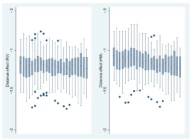
As mentioned above in this section I start by listing the regression coefficients of the 27 industries for all the 24 years 1296 (24*27) as indicated in Fig 1.2. The results obtained from HM and RV estimation methods are indicated in panel b and a respectively. In the graph below which depicts the distance coefficient obtained from the data a given line is a representation of a specific year for which the data was analyzed as indicated. From the representation we can see that the range of coefficients analyzed fall in-between 0.67- 1.73 notwithstanding the evidence of high heterogeneity between industries. Again, as we can see from the figure, time is not inversely related with the distance effect and this is consistent with several recent studies (Mayer, 2008; Disdier and Head, 2008; Anderson and Yotov, 2008; Egger, 2008; Boulhol and de Serres, 2008).⁵

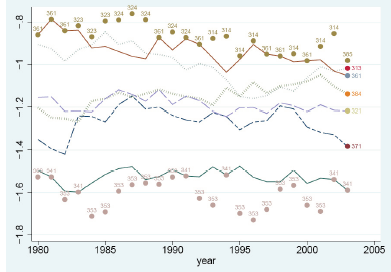
In the figure 1.3 the data analysis provides a clear trend of industry evolution in some sectors; the numbers indicated within the graph indicate the industry sector involved for the duration of years sampled, each year showing the sector with the minimum and maximum impact. In 1980 for instance the graph indicates that the sector that had the greatest impact was 369 which is “other non-metallic mineral products” while 341 “pottery” had the least impact; towards the end in the final year analyzed 341 “paper product” sector again had the highest and 365 “professional and scientific equipment” the least. Overall, as we can see 353, “petroleum refineries” was the highest scorer in values for the whole span of duration; while 314 “tobacco” and 361 “pottery” appears least impacted by the variable of distance compared to the rest. The line linking the industries is a measure of how closely the coefficients of the sectors are aligned which is a comparison between industries; in this case the indication is that the effect of distance across sectors is much or less the same except for some outliers such as sector 361, “pottery”.

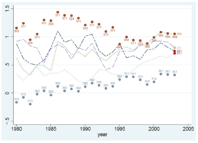
Where the only variable introduced in the estimation of freeness of trade is distance, it might be challenging to establish the extent that trade cost impacts on market access because of the similarity of the coefficients involved in these variables. To overcome this, use of other variables that lead to varied coefficients is recommended which are several in this study such as time distance; Fig 1.4 summarizes the impact of RTA across sectors. Based on the analysis it is evident that 371 “iron and steel” industry is the most impacted by RTA based on its coefficients, except for this all industries appears to be impacted in the same way across the board in general.

Additionally, it is notable that in the final years analyzed the coefficients for all sectors are predominantly positive exhibited by great variation within the specific sectors; this observation is consistent with RV method as well as HM method since the analysis shows evidence of variation between sectors and across time.

In determination of trade freeness between two-paired countries, the study relied on several variables to generate trade costs by way of proxy; thereafter the impact of trade freeness is calculated by summation of values of all importers. This is similar to market access measurement except for the lack of price index and demand functions that are considered linked with wage variable as shown (That is,

_ij instead of _ij )

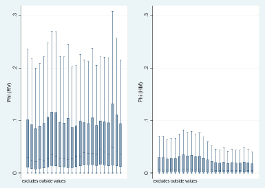
This model will be the tool that will be applied in determining market potential in subsequent sections of this paper; in fig. 1.5 the freeness of trade variable for each region compared in respect to method used (HM or RV) and time is indicated. In this case there is evidence that countries are less integrated with each other based on the pattern of distribution as indicated which appears skewed. Unexpectedly, there is no evidence of improvement of freeness of trade as one might anticipate considering the impact of globalization, although this could be attributed to the negligent variations present between sectors. Indeed, more detailed comparison of this analysis will indicate that there exist crucial variations between industries which cannot be demonstrated in these graphs because of space; in fact, extreme values have been excluded for the same reason.

When freeness of trade is compared between the two methods (HM and RV), there are observed differences such as the borderline effect, usually not measurable through RV method and in coefficients.

Changes in world economic geography

Coefficients obtained from distance variables indicate distance as among the major factors hampering trade despite globalization efforts that is recognized as influential in facilitating the same; nevertheless, this observation does not hold for all regions because distance on itself is dependent on other factors. In order to assess the similarity of country’s trade progress we rely on the market potential variable because it incorporates both aspect of market size and trade-freeness. Based on this Fig 1.1 can be interpreted since it presents the evolution⁶ process of 4 key sectors. The tone of the color is the code that indicates the rate of progress of the country towards trade-freeness or integration of its economy. Hence, dark colored countries are those making positive progress while light colored countries are those which has negative progress towards this end. Tattletale gray for instance indicate nations that have negative progress, light grays represent regions that are neither progressing nor backtracking on their progress while those colored in black have significant progress towards trade freeness. White color implies those countries that cannot be effectively determined essentially because they have missing values.

By looking at panel (a) which represents tobacco industry, it is clear that no significant change in ranking has occurred over the years; this is typical of an industry that is highly regulated which is always indicated by low-level dynamism which is consistent with present literature. In this case the barriers present in this sector relate to such issues like exorbitant taxations and controlled advertising. In panel (b) we have textile sector which mainly utilizes low technology level where there is evidence of robust progress by several countries such as India, China, Turkey, Mexico and Vietnam while few others such as Angola, Iran and Argentina have negative progress. The rest have largely minimal progress if any and constitutes peripheral countries such as Spain and Romania among others. This is a clear indication that proximity advantage can drive freeness of trade in the absence of benefits expected from low wage labor which has traditionally been attributed to the same.

But countries such as US and Brazil appear here able to weather the factors that hinder the freeness of trade which is attributed to their high level of internal demand; consequently, the wage evolution evident in the same regions can be attributed to reduced market access caused by factors such as low wage allure (Lu, 2007). Besides, these issues, it is likely that other factors impacting on trade could lead to the same outcome. Panel (c) indicates the “iron/steel” sector evolution which is generally considered medium level technology intensive (Lall, 2000; Zhu, 2005); data on this panel shows a couple of countries registering positive progress such as Spain and Canada. The last panel (d) comprises of professional & scientific equipment which is the first high-end technology savvy industry (Lall, 2000) that we encounter which Zhu (2005) describes as “exhibiting low product cycle”. In this panel, the generated values indicates crowds of spatial pattern that is dominated by most developed countries which have the highest progress based on rankings followed by countries in Asia. The reliability of the method used in analyzing data in panel (d) is collaborated by use of RV method which also generates similar results for market access correlated at 0.74 for all industries with the lowest correlation registered at 0.55 for several industries such as Beverages.

NEG Wage Equation at industrial level

Baseline regressions

This relate to table 1.1 below which lists elasticity values for various country’s market access; the level of confidence required to establish the required threshold is 0.1%. In general, the following observations can be deduced from the dataset in this table; one, is that only two sectors exhibit negative coefficients that are significantly high, in column 4 which are “machinery electric” and “machines”. Two, across sectors there are only 2 industries, “petroleum” and “tobacco” that have coefficients that cannot be described as significant for all estimations generated. By analyzing elasticities based on their significance and positivity, values that ranged from 0.48 to 0.05 from various sectors are observed; Leather products for instance has 0.48 while tobacco has 0.05.

Thirdly, the efficacy of HM method over that of RV is evident when the results of several columns are selectively sampled; in this case 1, 2, 5 and 6 because of the accurate estimates obtained by the previous method compared to the latter. Four, when using RV approach, it emerges that the coefficient is patterned in a way with those generated from market potential in column 5 being generally lower than coefficients obtained from market access. This can only be attributed to the method of application rather than internal demand considering that the same coefficients do not vary when the HM method is used. Because of the relevance of this analysis to the study more in-depth analysis on the same will be the focus of the following section.

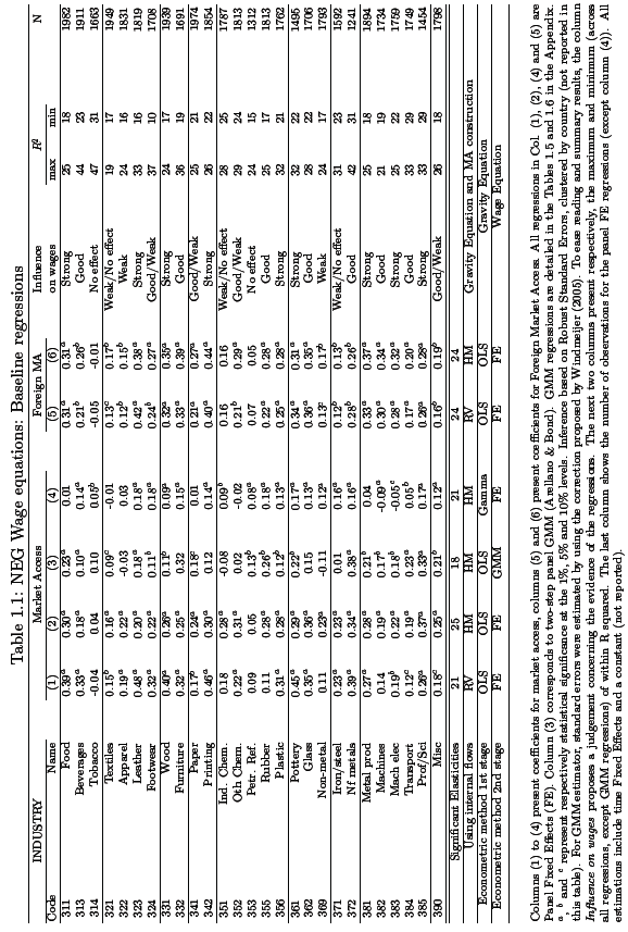
Across sectors there is evidence of correlation between market access and wage response that varies depending on the sector; in specific sectors, as much as 9, the coefficients obtained are consistent with the NEG wage model. In practice what this implies is that a 10% increase for instance on market access will lead to a corresponding 2 or 3 % on positive increase on wages as is the case in sector 383, Manufacturing of Machinery Electric. Additionally, 11 other sectors have correlation that can be categorized as average/weak; a good example is the Beverage sector which has strong coefficients but weak measures of market potential because of the exclusion of internal demand.

Lastly, in few sectors, 7 of them the coefficient obtained are not significant, consequently no correlation is found to exist between the two variables of interest. The Chemical industry for instance is one of the few sectors that have insignificant market access if any. In the column number 5 of the table, the values given are estimations obtained from GMM regressions for 9 sectors which in this case fail to determine if market access is a factor impacting on the cases. In regard to methodologies there are three notable issues that are worth mentioning; one is that RV method was established to generate market access values that were more elastic than values generated by HM method across all sectors.

Secondly, based on the data presented it is evident that market access and foreign variable have significant impacts on specific sectors notably “leather, petroleum, printing, textiles, machinery, iron/steel, paper and transport equipment”. Lastly, elasticity values obtained from market access is dependent on the proportion of values used in estimating market access; thus, GMM regressions in column 3 and FE benchmark (column 2) generates a different market access estimation unlike that obtained from column 4 that utilizes zeros from trade values.

Robustness Checks

Throughout the following sections, the market access estimations utilized were generated by HM method⁷, and when this method is not used the same will be noted.

• Endogeneity issues and industrial labor adjustment.

In determination of the market access several studies have highlighted the potential impact that endogeneity might have on the results particularly in regard to “reverse causality” which is a situation whereby drastic change in wage directly impacts on market access. This outcome is more probable where aggregate values of MA are relied in estimation of market access, however this challenge can be addressed through use of MA values that are sector-specific. This way any resulting external factors that shock the wages will be contained in the specific industry and consequently only the corresponding market access of the same industry will be impacted. Additionally, because of the use of FE estimation, bias related to omission variables are managed in the data but this doesn’t address the risk of bias emanating from observation of variables not fixed in time; as such use of instrumentation is highly recommended.

But use of exogenous instruments is hampered by their scarcity because in large they don’t exist, this is even more hard to obtain when the instrumentation is required to capture variation three-way; by industry, country and time. One such tool that can achieve this is use of Ø_ij summation among importers; use of this function is relevant for these purposes because it factors in all related trade costs obtained from gravity equations in calculation of the sector market potential without considering fixed effects affecting the same importers, and by extension their income. Since Ø_ij is also an indicator for level of trade integration present in two countries, then it implies that this function can be used to measure the remoteness of a particular region by way of proxy through summation of j across regions as described by Mayer (2008).

The phenomenon of endogeneity is also interrelated with other labor market factors such as adjustments impacting on labor and market access reactions both of which are not clearly documented. From this observation job mobility is explained as the reaction by workers to switch sectors by moving to other industries triggered by wage variation while international migration is also triggered by a similar factor but which occurs across countries within same sector. The impact of these both outcomes is overall reduction on market access in regard to wages.

To investigate the phenomenon of intranational (within regions) job mobility, I utilize several analyses; in this case I opt for the GMM estimator because it utilizes panel data that facilitate comparison of labor and wage adjustment. Based on the current literature I expect results to be consistent with study findings that indicate wage evolution is linked to decreased employment rates when labor adjustments across sectors is investigated (Artuc et al., 2007), or in fact free trade as Wacziarg and Wallack (2004) asserts. To explain this outcome several theories have been advanced mostly based on conditions affecting labor market such as legal frameworks, sectoral specialization and individual idiosyncracy among others (Davidson et al., 1999; Hasan et al., 2007; Kambourov, 2009; Artuc et al., 2007).

Just like other studies utilizing similar data, this study is limited in terms of data completeness in some sectors such as data on workers mobility between sectors or across countries (Hoekman et al., 2005); in such cases, the study recognizes the fact that employment adjustment maybe impossible to find, and not because it has not occurred (Bernard et al., 2003). Having said that, decreased response across sectors can also be attributed to industry-specific resilience that is typical of this characteristic; indeed, this problem has been addressed in several studies through use of lags paired for each variable in a bid to capture the progression and thereby effect GMM approach.

In implementing the GMM dynamic panel estimations, I adhere to labor adjustment procedures as outlined by Arllano and Bond (1991), Milner and Wright (1998), and Greenaway et al. (1999), the last two of which focus on effects of free trade on labor adjustments. In line with this, I apply two form of lags⁸ (one and two) to represent wage and employment which I treat as regressors, and then utilize the two-step GMM equation discussed earlier on the data already differenced. In this process market access is assumed to be predetermined (used when already lagged by 1 year) to ease the analysis.

This gives us the variable as

ln w_i,t-1 = ψ₁ + ψ₂ ln MA_i,t-1 + ψ^’ ln w_i,t-θ + ψ^’ ln L_i,t-l + c_i + µ_i,t (1.15)

with l = {0, 1, 2} and θ = {1, 2}.

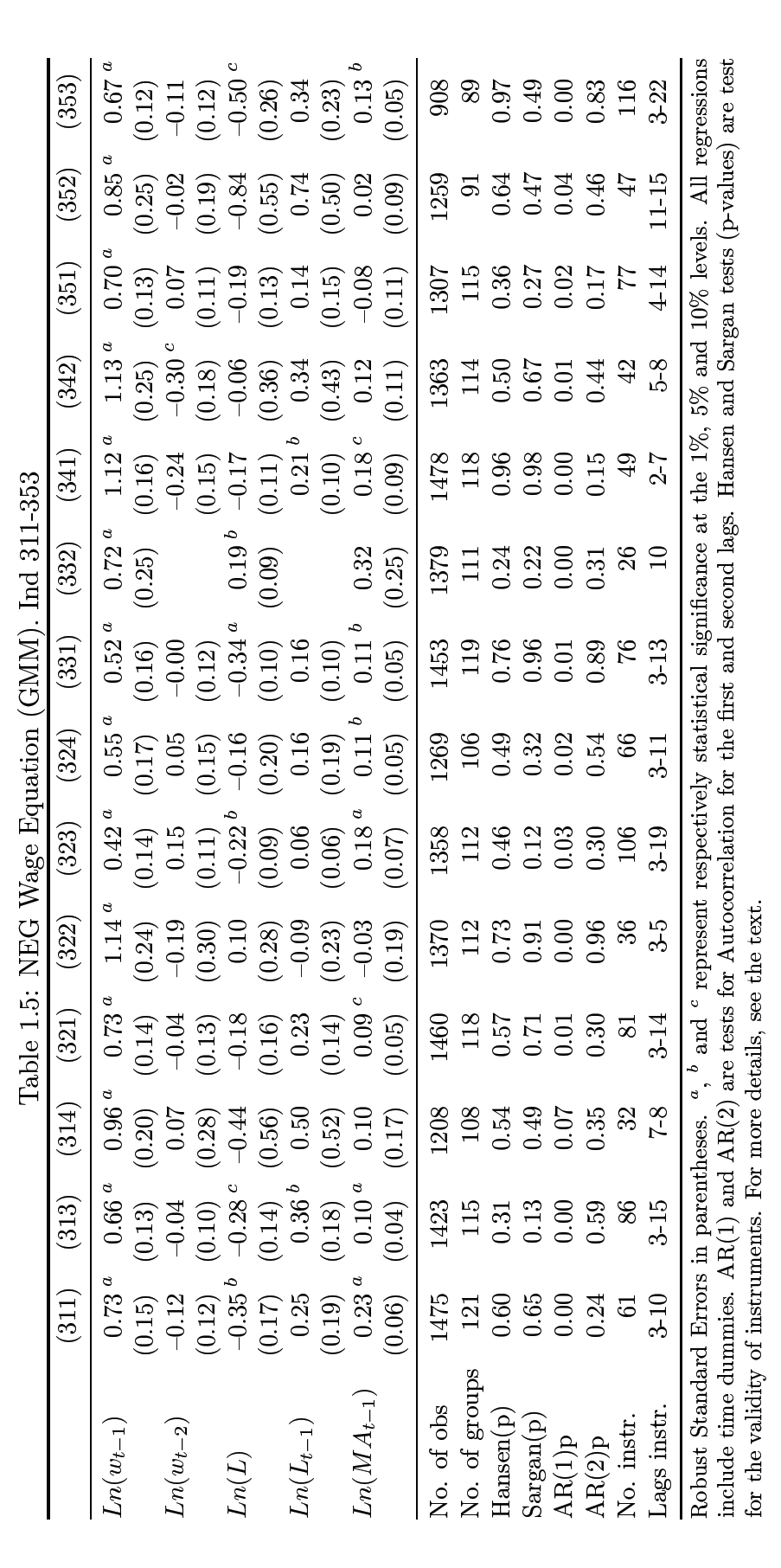
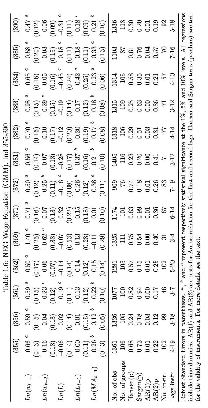
In this case, the purpose of the above equation is used by the GMM to factor out the fixed effects ci for countries analyzed; by design a correlation is developed for two of the functions, the error term (µ_i,t – µ_i,t-1) and the differenced-dependent variable previously lagged (ln w_i,t-1 – ln w_i,t-2). In estimation using this approach, 2^nd and subsequent lags on values can be reliably used as long as the results given by this µ_i,t residual are not used as correlation ⁹. The values generated here are indicated in table 1.5 and 1.6 (appendix section).

The regressions obtained here have only 1^st order correlation for error terms instead of the 2^nd order correlation which is the recommended standard level of validating instruments used. So, I utilize the Hansen and Sargan test to measure again the same instruments validity, all except one (industry 341) are certified as valid; the instruments assessed are those that have 3^rd variables. Because of the extensive time dimension that characterizes the panel data that I wish to analyze which cannot effectively be managed by a single instrument, I rely on guidelines advanced in several studies for merging instruments to overcome this hiccup and address dimensionality (Calderon et al., 2002; Roodman, 2006; Beck and Levine, 2004).

The results of wages on 1^st lag indicates high significance which implies persistence in the industry which is consistent with our assumptions while the second variable, employment levels lagged or otherwise also indicates evidence of significance across 13 sectors. But following adjustments, the values for all 1^st lags in employment level variable are all registered as negative.

The resulting coefficients generated from market access can be used as the basis for checking the accuracy in panel FE even though the data in this panel is often inaccurately estimated. Regarding elasticity in coefficient results, this was found to be in the range of 9% “textiles” and 38%, “non-ferrous metals”; this is consistent with results of elasticity variation at international level as detailed by Boulhol and de Serres (2008) and Head and Mayer (2006), and also at intranational level as determined by this study earlier on and Hering and Poncet (2009).

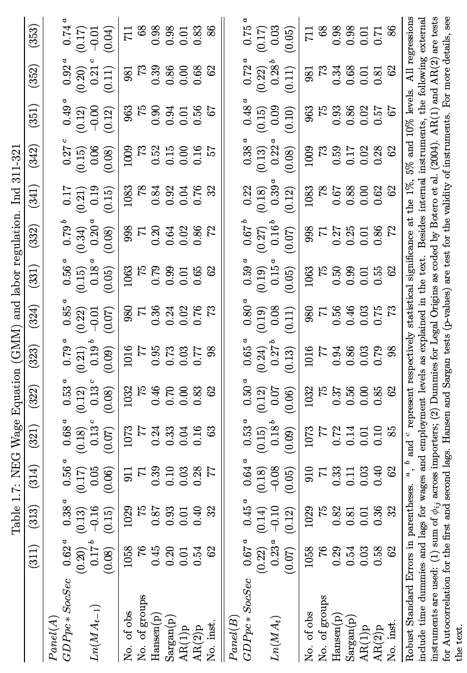
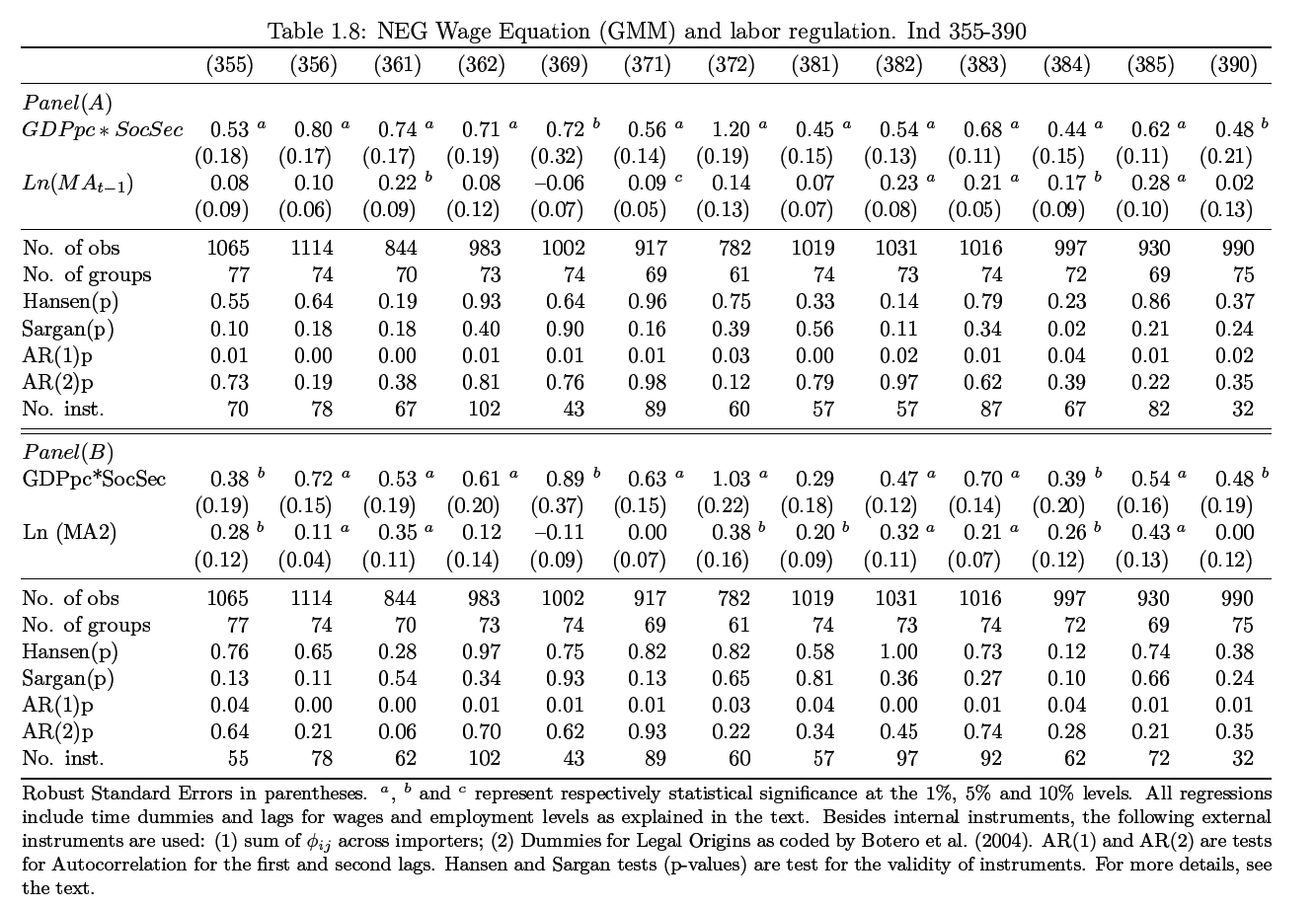
Because of data limitations and scarcity of literature review that investigate the impact of wage persistence within the NEG model, this study will only present exploratory findings that can inform future research on this phenomenon, more so because it is a subject that is beside the point of this study. A study by Botero et al (2004) contains data of 85 nation’s labor policies which the author suggest can be used to explain the variable of wage if differentiation of key policies such as security law is computed. Because, the resulting differentials performed do not have the element of time variation I introduce this element by proxy through linking the variables with GDP per capita which has been found to be correlated with the level of development of a country by the same study.

Thus, GDP per capita is in general found to be more meaningful as a proxy for time variation in developed nations, which also gives rise to other challenges such as the inability to sift through the variables and compartmentalize the impact caused by either GDP per capita or by labor regulation given their endogeneity. To address this, I introduce a legal origin instrument and the results are as shown in table 1.7 and 1.8. where the regression values are lagged as previously detailed in equation 1.15. In the tables two coefficients are presented, labor regulation and market potential. In panel (a) regression results for market potential already 1-period lagged are presented while panel (b) lists coefficient results for the same variable that are not lagged. As can be observed several of the regression values are at the borderline, barely certifying the validity test; the purposes of their inclusion are two.

One, they verify the completeness of the data and secondly, they demonstrate how challenging it is to obtain GMM regressions from a small dataset. The results indicate that coefficient for market potential ceases to be significant for a number of sectors that have previously registered high significance such as “beverages”, “plastic” and “footwear” among others. Additionally, there is evidence of significance in regressions generated from Social Security Index when GDP per capita is linked, while this might not be accurate in terms of values, a general trend can be inferred. In conclusion therefore based on these analyses it is clear that the relationship between economic geography and labor regulation can and should be explored with more reliable tools and approaches.

• Spatial adjustment.

By considering the wage equation demonstrated earlier, the international spatial adjustment values appear to be captured within the price variable which would ordinarily be consistent with factor immobility theory. But this could also be attributed to the outcome of industries decentralizing characterized by firm relocation because of the globalization effect across countries. So, to clarify which is which, one reliable approach will be to assess whether the market potential is in anyway correlated with employment distribution across sectors (regression obtained in the course of this analysis are not presented here but can be presented on request). In 6 of the sectors, significant level of coefficient was established; in half of these sectors (3), the industries with high coefficients are those that have indicated a tendency to relocate over the years i.e. Footwear (0.27), Leather (0.25) and Apparel (0.16), coefficients indicated in brackets. The remaining three have coefficients of 0.06, 0.12 and 0.06 and are Plastics, Beverages and Non-metals respectively; these results would indicate that use of labor is not indicative of quantity response.

• Wage equation with human capital controls.

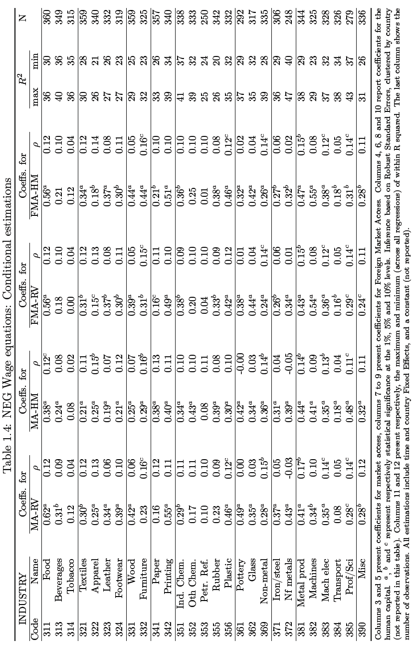
In this section I apply similar regression estimations as above, but in this case a control variable is introduced (human capital levels); the generated values obtained plummets to about 300 which is attributed to the fact that data pertaining education variable is limited both in years (5 in this case) and across countries. This section summarizes only the key coefficients observed from this data. In table 1.4, the values listed are of several categories and include; levels of significance, coefficients, R² for each and every regression listed, RV and HM methods values that are disaggregated based on foreign version and total market access. This is necessary in order to differentiate the regressions generated from total market access which is the interest of this analysis and is listed in 1.6 and 1.7. Here, the results are plotted against each other to depict the pattern of the relationship; coefficient against industrial regression as shown by the points which represent the level of magnitude where MA and human capital level are for horizontal and vertical axis respectively. Unfilled circles are for MA coefficients that fails the test of significance set at 0.05 level of confidence.

The RV method, values are indicated in Fig. 1.6; the variable of market access is better understood when worker skills are controlled; in seven of these industries listed the elasticity attributed to market access are not significant (these are Rubber, Refineries, Petroleum, Paper, Tobacco, Other chemicals and Transport equipment). The data also indicates evidence that substitution between variables is possible; this is evidenced by the fact that wage is found to be linked to level of education for some specific sectors such as Professional and scientific products. Similarly, and consistent with our expectation industries such as Pottery do not appear to be correlated with level of education when it comes to wage, but the same is significant towards market access.

Also notable about the data in this case is the inaccuracy exhibited in most of the coefficients listed herein which is nevertheless expected for several reasons; first this could be related to the limited data, inherent weaknesses of the measurement tools, and incomplete dataset. Secondly, the need to measure the impact of school level through the wage variable could have led to less reliable values since the same is better captured by another variable, industry growth as Ciccone and Papaioannou (2008) documents.

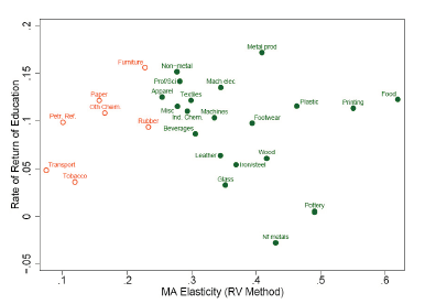
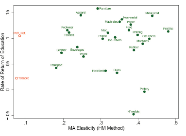
Figure 1.7 shows that skill sorting has negligible effect on values generated by HM method; additionally, it is also evident that all of the industries except 2 have positive coefficient on regression values generated from market access.

• Controlling for the geography of production costs: Supplier Access.

The wage variable and how it is impacted by trade when analyzed through NEG mechanism can be further understood when it is linked to the Supplier Access (SA)¹⁰; the SA is an indication of how strategically placed a firm is in a particular industry that has many competitors (producers) impacting on the resulting costs. Ideally, the partial equilibrium holds that the variables mentioned above interact together in influencing the profit returns in an industry. But in practice, there are two distinct phases of geographic concentration that are known to emanate from the process of globalization; first, trade costs gradually decrease leading to firms agglomerating towards regions that have high demand. Since suppliers are also interested in reducing trade costs similarly, they are attracted by industries in these regions and they follow suit. This status quo will remain as long as the market is able to sustain the trade; this balance eventually changes usually tipped by the globalization triggering a redispersion of the same industries towards the periphery.

The redispersion in this case emanates from the rapidly depreciating trade costs, now occurring in the periphery compared to those found in centers of demand which motivates the firms to relocate again. This entails the 2^nd stage of geographic concentration; as a rule of thumb firm relocation in this case will be influenced by “geography of low costs” rather than the trade costs related to demand centers. Indeed, a study by Fujita et al (1999) asserts this and provides a simulation model that predicts the sectors that are most likely to go through redispersion process in which they identify three factors that characterize such firms i.e. labor intensive, inefficient input-output linkages and those that are final demand oriented. Once this have redispersed, interlinked firms that are closely interrelated in processes (usually those that require inputs from these firms) follows suit. Consistent with earlier observation in which we saw SA to be correlated with wages, another theory which hypothesizes zero profits where international migration is nonexistent is observed to be valid. Thus, to evaluate this I will rely on the variable of wage as my indicator of determining industries that respond to supplier access and the extent that this influences the price variable for market access. On analysis, it becomes evident that market access and SA are clearly correlated at national level, which makes it impossible to delink their effects from each other thereby calling for sector-specific data to address this challenge.

Because the SA measure can be developed for regression purposes, I set to have one in place by utilizing the functions of FXi and FXik that denotes total gravity regression and gravity regressions per sector respectively while using the same procedures outlined in developing market access measures. The results indicate that use of supplier access that is sector-specific will be ineffective since the cost is a function for all the sectors; besides, regressions performed in Panel FE fails to be significant regardless of the approach taken. In light of these limitations I follow Redding and Venables (2004)¹¹ procedures and design another version of SA that is able to pool data from all sectors and therefore better positioned to give reliable data when coupled with RV technique.

This time in panel FE, significance is established in 14 of the sectors implying dissociation of wages across industries; further analysis that combines SA, regression and sector-specific market access more data that has interesting implications are generated. First, we realize that SA remains significant in 8 of the sectors, in two of these industries (paper products and textile) the only significance established is on the variable of “proximity to suppliers” which imply that trade costs based on demands do not influence location for these sectors which is consistent to literature review discussed previously. Secondly, there were category of sectors that recorded high significance across the two variables; these included those related to textile such as Footwear and Leather in addition to others such as Metal products and plastic.

Lastly, the evidence for significance level is inconclusive for two of the sectors because of the conflicting results given by the different techniques which could imply borderline coefficients; these are Science equipment’s and transport. In conclusion, the general trend of coefficient significance indicates evidence of supplier access in most of these industries, but because the significance of coefficients is directly related to trade costs the results should be validated because of the limitations of this data. In any case the various methods of measurement have shown great variability in measuring this variable¹² as we have seen which will require development of reliable instruments whose accuracy are not dependent on data.

• Summary on robustness checks.

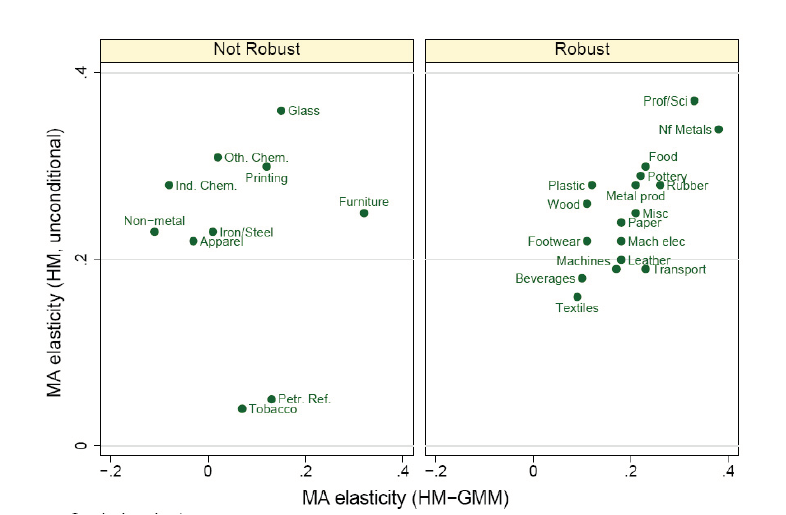
There are two observations that can be inferred from data analysis undertaken on previous section of this paper on robustness; one, is that among the two methods outlined for estimation of market access, HM approach appears to be most effective. Two, the HM method which we find to be reliable illustrates that 16 of the sectors (listed previously) have significance results that indicate wage is impacted by the market access; further analysis using Panel and GMM techniques generates various coefficients (listed in Fig 1.8) on respective columns of table 1.1. Columns on the far right indicates coefficients that remain significant despite the choice of method used, and then simulations of the result as we shall see shortly.

How policy changes could affect the economic geography and wages

The aim here is to simulate change in wages¹³ that originates from the effect of market access; this requires a working method that enables a “comparison of country level impacts versus country-industry-specific impacts” as Mayer (2008) suggests. Similar to an approach utilized earlier, the RTA (which is one of our working variables) dummy is pegged at 1 where both partners are members; from this we can see how the coefficients associated with this variable evolves with time. As above, the dummy is again fixed at 1, for our 2^nd variable WTO when both parties are members to the organization; when the results for the two are analyzed we note that both impacts on trade costs.

This has two implications; because trade costs directly influences firm choice of locations, the results is that economic geography is also shaped, and eventually the level of wages capped for each region. To estimate the resulting impact one year is chosen (2003) and HM method used for analysis. One approach requires the HM method to be calibrated using values of labor that are proportion to production β and substitution elasticity σ; the equation presented by Mayer (2008) is β =0.2 and σ=5. The values generated from this simulation model are listed in table 1.2 in 4 of the columns, 8, 7, 4, 3 two of which shows the average impact for all regions (3 and 7), while the other two (6 and 8) indicates values loss across sectors.

Further, analysis of results shows that WTO is indicated as a more valuable partnership compared to that of RTA given that wage variable is more impacted by the earlier, this is consistent with a similar analysis by Mayer (2008).

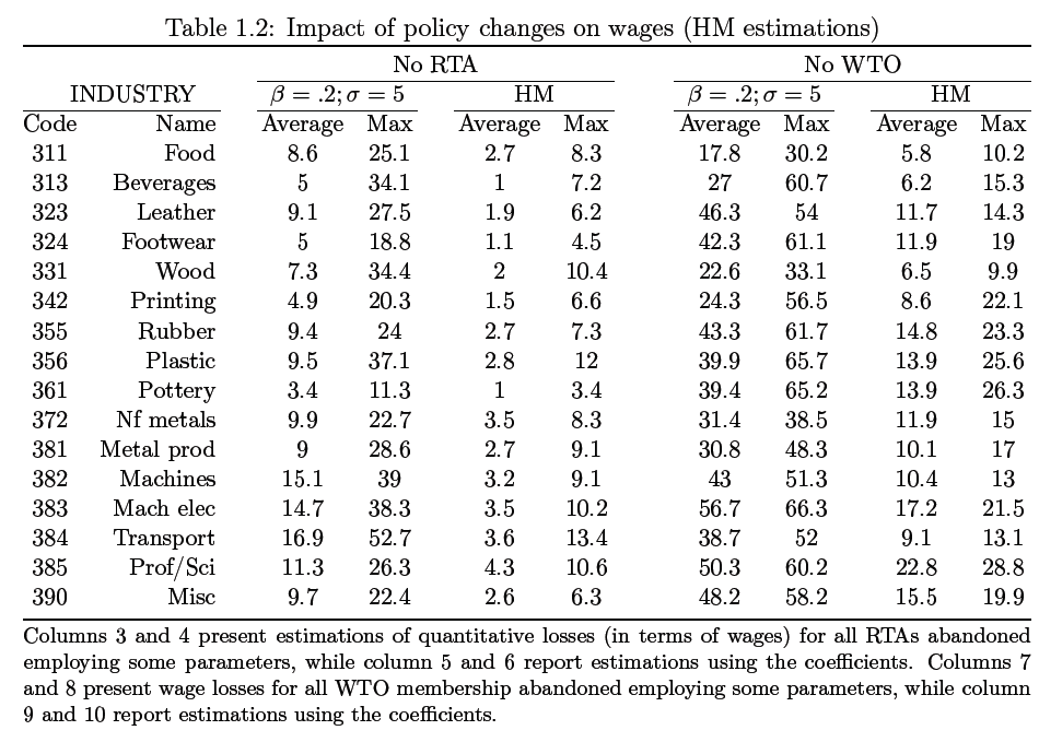
Because the choice of calibration used for these purposes is problematic and clearly inaccurate, I utilize the coefficient values of table 1.1 column 4 to overcome this challenge. By using these values, I am able to generate realistic coefficients despite their negligible values for both variables that I wish to compare as displayed in table 1.2; RTA results are in columns 5 & 6 while WTO are in 9 & 10. In general, the range of losses occurring across sectors based on these results is indicated to be as much as 4.3% starting from 1% among RTAs and notably higher in WTOs at 5.8%-22.8%.

Additionally, the distribution of losses indicate a patterned trend among countries evaluated, with those suffering significant losses being characterized by factors such as (a) small land area km² and low GDP (common in African countries) (b) peripheral countries and landlocked or developed economies that have withdrawn from WTO and RTA membership (c) peripheral countries with sectors that are mainly high-tech (applicable to RTA only) and finally (d) emerging nations (WTO for only). In this analysis, the data doesn’t support evidence of losses attributable to industrial specificity.

Concluding Remarks

Throughout this paper we have investigated in great detail how the NEG model is shaped by the market access variable; we also evaluated the regressions values generated from the variables using the market access through different proxies; in this case manufacturing wages and employment. Two approaches well documented in literature sources were also utilized in estimation of MA; one is the gravity equation of trade flows whose inputs were 24 yrs, 27 industries and 2 methods, generating 1296 regression values. Secondly, the Panel linear regression is used which utilizes MA variable to explain the impacts of employment and wages; based on the model developed significance is established for 16 of the industries.

Additionally, by using alternative approaches to cater for market access the study was able to establish an inverse correlation between the wage equation and employment meaning that relocation cannot singlehandedly be expected to shape market rewards. The results failed to show significance in Supplier Access and the influence of labor policies on MA as would have been expected and future studies should explore this outcome further. We realize based on the evidence presented that agglomeration and redispersion of industries is essentially a slow process that is evidenced by the case of Asia where it has been taking place over 25 years. In summary, we deduce that trade policies have significance influence as highlighted in section 1.4.4 while RTA has great impacts in several of the industries of peripheral countries that are considered high-end. On the other hand WTO impact is only significant and limited in regions that are considered emerging economies without regard to sector specialization.

Appendix

Theoretical model

Following Dixit-Stiglitz-Krugman model of trade, I hypothesize that elasticity is constant for all product types where each product variety is matched to a specific firm that is within an industry characterized by a competition monopoly. Since, both consumers and producers are dispersed across regions, I employ the function of τ_ijs ad valorem trade costs to every pair of countries (i & j) for a particular sector s; where the s function is not included the implication is that industries in those countries are not correlated.

In later sections of the paper, this model is further customized to incorporate industry-linkages related to cost function (SA) while the demand-linkages retain their independence. Consistent to a particular research study by Zeng (2006) I inch further and hypothesize that workers movement between industries is negatively impacted by factors such as labor regulations that emanate from human capital variable. So in this section we consider a scenario in j countries where economy is two-sector; in A-sector the features include perfect competition, stable returns and nonexistent trade costs. As we had pointed earlier, such an A-sector will balance the opposite features evident in sector-M and in the process nurture specialization. On the other hand, because M-sector experiences trade costs for instance, agglomeration of industries is facilitated by this sector. The outcome of this is well demonstrated by the Cobb-Douglas function while utilizing the Dixit-Stiglitz sub-utility for the M-good; µ denotes the regional income proportion.

Ui =; 0<µ<1(1.16)

Mi for this equation represents region i data of sector-M consumption index; the variety in this case is for all N products captured together with qji (v) function that denotes “demand of region i for the vth variety coming from region j” (Baldwin et al, 2003). Since, each industry can be matched to a specific variety it is possible to explore the relationship between any numbers of varieties against firms nj based on the limits given by CES for any paired variables.

To determine the demand for a given country j originating from i necessary to estimate country-specific MA which is my aim in the next step, I rely on profit variable maximized for each firm; the demand denoted by qij (v) in this case is a function of three values, the Yj, pij and pj (regional income, CIF price and price index) respectively. The change in trade costs across regions, i and j for instance can be demonstrated by a model where pi is the mill price and the price is given by p_ij = p_i τ_ij :

q_ij = µY_j(1.18)

The P_j^1-σ, is the price index and serves as an indicator of the market size since it estimates potential suppliers by utilizing data from trade costs, price of goods and substitution elasticity. For this reason, the price index is also viewed as an estimation of market crowding indirectly since it is characterized by low or high product prices depending on the level of firm concentration. In evaluating the supply model, only the data from the variable of labor are utilized as was discussed in chapter 2.

In the equation below, the M-sector returns are modeled by the function of fi and mi which is the fixed costs for each firm and marginal cost respectively; using this model profit for a given industry is estimated by,

π = p_iq_i – m_iq_i – f_i (1.20)

When profit is maximized, a mark-up that is constant is finally achieved as indicated.

p_i

(1.21)

When demand function is introduced (model 1.18) together with gross profit function given by

π_ij = p_ijq_ij/, it is possible to estimate profit in a given market by applying;

By revisiting the function of phiness of trade Ø_ij advanced by Baldwin et al to model an equation of calculating net profit for region i and all regions j

As shown above, MA is the Market Access where Mai denotes the summation of demand directed towards region i, which is then averaged by a coefficient that measures the accessibility of market j through Ø_ij and P_j^1-σ. This is informed by the theory that states in every firm is inclined to earn the same profit from a given market. Finally, a model that mathematically links MA to costs is developed which is an iso-profit equation.

Additional tables

Footnotes

1. Redding and Venables (2004) develop a model with labor and vertical linkages in a Cobb-Douglas function. Baldwin et al. (2003) present models with capital and labor. Head and Mayer (2006) introduces differences in Human capital across regions. The Redding and Venables’ version is developed in Chapter2.
2. Given the assumptions in relation to the A-sector, there is interregional price equalization for this good, and wage equalization for the unskilled workers as well. This allows to take the A good as numeraire:
3. All regressions are at industry level, estimated for each year. Subscripts for industry and time are omitted, except for RTA and WTO variables, that can be time-varying.
4. Great circle distances are used, which only require latitudes and longitudes. Head and Mayer (2002) argue that using different methods to calculate the bilateral distance can affect the estimation of the other coefficients. They propose a measure that refines the great circle formula adding weights. It is refereed in the dataset as distance-weighted (distw). This variable uses the distribution of population inside each country.These authors also develop an alternative measure of distw that introduces an additional parameter to reflect a sensitivity of trade flows to great circle bilateral distance, which is often -1 in empirical estimations (More details in Head and Mayer, 2002). I also calculated market potential using these measures. I do not report these results here, because they are quite similar to those found for simple great circle distances.I prefer the simplest method because latitudes and longitudes are available for all countries, which is not the case for internal distribution of the population.
5. Several explanations have been proposed for this result, among others, the surge of capital/labor ratios (Egger, 2008) and substitutability of goods (Berthelon and Freund, 2008). Siliverstovs and Schumacher (2008) report falls in distance coefficients with industry-specific regressions, only for OECD countries.
6. Rank evolution is the change in gained or lost places in the market access hierarchy, relative to the United States. Values are normalized as deviations from the mean across countries, and they are grouped in 5 classes. The middle group is comprised between the mean +/− 0.5 standard deviation, and the next groups are delimited by 1 standard deviation. Blanks correspond to countries with no data.
7. In all regressions presented in this study, I eliminate extreme observations below (above) the 1st (99th)percentile of the wage distribution. Results are robust to this change. They are also robust to: (1) consider only countries with more than 10 observations in a specific industry, (2) discard the high values of market potentials of Hong Kong, Macao and Singapore and (3) discard countries that entered in the dataset later in the period (e.g., former communist countries). Finally, I checked the stationarity for the series of wages and market potential by using the Fisher-type test for panel data developed by Maddala and Wu (1999).This is a non-parametric test where p-values from individual unit root tests are combined in a single statistic. I consider models with a simple random walk (without drift) and with a random walk around a stochastic trend. In the case of market potential, only for one industry (341), the null hypothesis can not be rejected in one variation of the test (the other strongly rejecting nonstationarity). For wages, there are four industries where both tests suggest nonstationarity (352, 353, 361, 372). Consequently, caution is needed in the interpretation of results for these four cases. Results from a variation of GMM (System GMM) suggest that market access is not significant for the first three of them. Industry 372 did not passed the tests required to obtain consistent estimation using System GMM.
8. In one case (industry 332), the full specification of employment and wage lags results in rejection by the mentioned tests, but a version with only the lagged term for wages (lnwi,t−1) and the contemporaneous term for employment levels (lnLi,t) passes the tests.
9. Additionally, the assumption of weak exogeneity must be valid, i.e., current explanatory variables maybe affected by past and current realizations of the dependent variable, but not by its future innovations.
10. I will only comment main results. All regressions are available on request. I will not comment regressions on Tobacco or Petroleum Refineries because they gave similar results to all other previous results, that is, no wage response at all to the NEG variables.
11. In this case, trade regressions using all manufacturing are performed, and the exporter fixed effects recovered are country-specific, but not industry-specific.
12. I also explored a weighted Supplier Access (See Chapter 2 for the methodology, in the context of a cross-regional study) where all industry-specific exporter fixed effect FXik are considered in a composite indicator. Weights are the share of expense devoted to inputs, taken from an input-output table. I employed the USA matrix. Results did not improve (no more than 8 industries exhibited some significant impact of SA), possibly because the USA matrix is not correctly representing technological levels for all countries.
13. Simulations in New Economic Geography models have followed two paths. A group of studies are interested in the long-term consequences of reduction in trade costs on agglomeration patterns. These works emphasize migration or FDI as adjustment channels. Some examples are Forslid et al. (2002), Crozet (2004) and the Chapter 3 of this thesis. The second line of research (followed here) is interested on the spatial transmission of the shocks in the market access (or its components). These simulations focus on wages (or GDP per capita) at intranational (e.g. Hanson, 2005, and Mion, 2004) or international level (e.g. Mayer, 2008).