Introduction
Background
Resistivity logging constitute a way of well-logging by which there is the characterization of rocks or sediments that occur in boreholes through the measurement of the electrical resistivity. The so measured resistivity constitutes a very significant property that expresses the potential of a material to opposing an electric-current’s flow. This characterized property is measured through the use of 4-electrical probes for the elimination of resistance against contacting leads. It is absolute that the running of the log has to be in holes that contain electric conductive water/mud (Zhipeng et. al., 2007; Herbert et. al., 2008). Quite often, resistivity logging has been made use of in exploring minerals as well as in the drill of water-wells- however it has found the most appreciated application in formation-evaluations as regarding oil and gas well drills. A majority of rocky-materials are insulated in nature, but the fluids which enclose them are usually conductors. It is noted that:
‘Hydrocarbon fluids are exception because they are almost infinitely resistive’ (MacCallum et. al., 1998, p.12).
It is further noted that:
‘When a formation is porous and contains salty water, the overall resistivity will be low. When the formation contains hydrocarbon, or contains very low porosity, its resistivity will be high’ (MacCallum et. al., 1998, p.14).
These variations have necessitated various approaches towards drilling- and quite an number of resistivity tools which are made up of varying investigational lengths have been put into use for measuring formations of resistivity. Ordinarily, during drillings, the drill-fluid invades the formation/changes occurring in the resistivity and the measurement is done using tools that work effectively at invaded zones. Roberts et al., has suggested that:
‘If water based mud is used and oil is displaced, “deeper” resistivity logs (or those of the “virgin zone”) will show lower conductivity than the invaded zone. If oil based mud is used and water is displaced, deeper logs will show higher conductivity than the invaded zone’ (Roberts et al., 2007, p. 29).
The study further notes, ‘this provides not only an indication of the fluids present, but also, at least quantitatively, whether the formation is permeable or not’ (Bittar and Rodney, 1996). The decision of what resistivity tools to employ for drilling has always been one met with quite a lot of difficulty by petrophyscists (tehehe). But generally, it is accepted that an induction toll is most appropriate for lower resistivity formations that are drilled using fresh/non-conducted mud. In this regards, later/resistivity tools have been employed for optimal results at varying conditions. One significant effect to put into consideration during the period of making a choice of a tool for usage has been the contrasting of flushed-zone-resistivity (Rxo) which has to be in line with an actual formation resistivity (Rt).
Over the years, the use of laterolog tool has continued to express difficulty in time estimation of actual formation-resistivity particularly at instances whereby Rxo may be higher than Rt. Hagiwara noted that:
‘This effect, though well known, still seems to catch petrophysicists by surprise and can cause serious errors in the formation analysis. Comparing measured tool response to forward modeling results helps explain the measurements’ (Hagiwara, 1996, p.14).
Categorization of Resistivity Tools
Logging-While-Drillings (LWDs) wave propagating resistivity-tools have been put to use in measuring phase-shifts as well as in attenuating electromagnetic waves that occurs within 2 receiving coils. The categorization of quite a number of resistivity tools follows a numbering of transmitter-spacings as well as the frequencies these tools operate at. The measures according to Anderson et al., (1990) would usually be processed to generate estimated numbers which would comprise clear resistivity for targeted surrounding formations. Ordinarily, measuring of phase-shifts and the measuring of attenuating units over 2 receivers is done through individual evaluations of apparent resistivity. The computation of resistivity is possible as stated by Meyer as:
‘…from either a single phase shift or single attenuation measurement, [and] an assumption needs to be made as to the value of the dielectric constant’ (Meyer, 1998, p.3).
Barnett and Meyer have further identified that:
‘Often this takes the form of a resistivity-dielectric constant relation, and different relations are used throughout the industry for the various tools’ (Barnett and Meyer, 1991, p.67).
These resistivities have been referred to as “dielectrically constrained” (Meyer et al., 1997). Meyer et.al., (1994) have noted that in specific terms, resistivity tools are used for measuring formation resistances to specified applied electricity current- perhaps, clay formations/sands that comprise high salinity would always offer lesser resistivity, where as sands that comprise freshwater would naturally constitute high resistivity values- such as it is the case with hard-rock/dry formations.
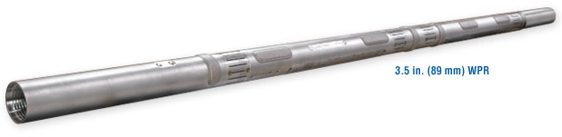
Apart from inductions, every other resistivity tool is an openhole tool which requires fluid in its wellbore running (Wu and Wisler, 1990). The running of the induction-log is achieved with the help of air holes as well as a non-metallic case. An APS is shown in Figure 1.1 below.
The general Tool Sizes and Maximum Dogleg Severity for the APS in Figure 1.1 have been given by Meyer (1998) as shown in Table 1.
Table 1. The general Tool Sizes and Maximum Dogleg Severity for the APS (Meyer 1998).
The tool is effective with:
- Power requirements: Low operating power for maximum battery life;
- Designed to run on 2x/3x batteries (10 cell DD) or 0x/1x/2x battery and turbine alternator; and
- Tool Programming and Data Dump port: Hatch cover for easy access via an intrinsically safe connection to allow tool programming and memory dump. Memory data dumps and tool programming can also be performed when the tool string is disconnected from the resistivity via the tool string lower end (Meyer et al., 1997).
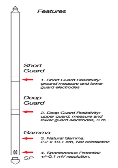
Figure 1.2 presents a 9076- Dual-Resistivity-Tool: this tool is capable of recording natural natural-gamma, self-potential, deep and shallow guard-resistivity (Hagiwara, 1996; Meyer, 1998). According to Meyer:
‘The measurement of formation resistivity at several different depths of investigation allows a correction to be made for the effect of mud filtration- an estimation of the depth invasion may also be obtained’ (Meyer, 1998, p.23).
Aim of the Study
The aim of this paper is to elaborate of factors that affect resistivity-tools – special attention would be paid to the functionality of multiple-resistivity tools (MPRs) and how they relate to multiple-propagation resistivity.
Literature Review
Effectiveness of Resistivity Tools
Resistivity logging is noted to constitute a way of well-logging by which there is the characterization of rocks or sediments that occur in boreholes through the measurement of the electrical resistivity. This so measured resistivity according the Herbert et. al., (2008) constitutes a very significant property that expresses the potential of a material to opposing an electric-current’s flow and has been put to practical use at several places itemizing a number of credits to the usage. Without the applicability of resistivity tools to drilling, at some points once in a while, there have been a number of challenges. For example from work conducted by Herbert et. al., (2008) at Long Beach in California, it was realized that there was difficulty encountered in drilling/exploiting leftover sites that existed in Old-Wilmington fields for more than sixty years.
However, the challenge noted by Herbert et.al according to Zhipeng et.al., was overcome through utilization of emergent technologies as well as through sidetracks of existent wellbores that comprised horizontal laterals for capturing of hydrocarbon-reserves which could be recovered in an non-economical way using well known conventional approaches. Very recently developed technologies that where adopted for used at that site included 3-D geologic-modeling, geosteerings in thin-beds and modeling-the-Logging-While-Drilling (LWD) (Zhipeng et.al., 2007).
Measuring propagation-resistivity could be altered by invasions, varying dielectric-permittivity, eccentricity, as well as thin bed. Considering instances whereby there are reasonably high levels of dips, an adjacent bed or a formation-anisotropy becomes an appreciable factor for considering log responses. Using multiple-spacing or multiple-frequencies with propagation resistivity tools becomes an enablement for calculating multiple-independence sets of defined vertical/horizontal resistivity. Further more, the identification and quantification of anisotropic technology becomes very helpful in the determination of more boreholes as well as formation effects.
The study was also conducted by Bittar and Rodney (1996) where the generation of determined location formation-boundary relating to horizontal-well boreholes was achieved (Hagiwara, 1996). The achievement was credited to the fact that utilized models were dependent on structural interpretations as well as on located formation-pos which reflected an indication of the information provided by the LWD (Hagiwara, 1996).
However, according to Meyer (1998), the case-history is an illustration of limits placed by short-normal and deep-induction-data that could be expressed in a curved form particularly for the generation of forward-models used in geosteering and isotropic-LWD limitations used in forward-modeling-programs whereby relative-dip could reason high such that it would be utilized for anisotropy for creation of momentous impact on documented LWD information (Meyer, 1998).
The effect of anisotropy on LWD/wireline resistivity measurements has been observed (Meyer, 1998) under the conditions that the effects, which may be as a result of alternations in the bed differences of the resistivity/variable saturations of the fluids around the region of the beds could impact on the measurement of the resistivities more than what is the actual data contained on such resistivity. When this is the case, the anisotropy assumes a vital place in terms of making available reliable data which may have a relative-dip of sixty degrees or even more, and subsequently there is the comparing of information obtained from offset-drilled wells that have a reduced dip. The capability for extracting the horizontal-component (Rh) as well as the vertical-component (Rv), following the measurement of resistivity using anisotropic formations has become essential. A forehand awareness of local vertical/horizontal resistivity-ratios permits for adopting of greater and easier understood models for forwarding resistivity even before a horizontal-drill well is considered.
The possibility for having a successful geosteering in existent well is a function of how effective the entire model has been put to effective usage and the quality of skills that the geosteering-engineer puts into using during the process. When a dual-frequency is introduced, Multiple-Spacing-Propagation-Resistivity-Tool (MPRTM) (Anderson et al., 1990) would the produce the capability that would direct the measurement of the formation of the anisotropy using the available information on the comparative dip. The tool used in this case utilized 32 varying raw-phases as well as an amplitude-measurement that uses 2 varying frequencies (2MHz/400kHz) and 4 transmitters which according to Zhipeng et. al., (2007) are said to be ‘long spaced array with a 35” spacing to the mid-point of the receiver pair and a short spaced array with a 23” spacing’ (Zhipeng et. al., 2007, p.98). Considering the configurations of the 32-raw values, there could be a processing of the values in order to generate eight completely compensated phases that would vary as well as attenuate resistivity (Meyer, 1998).
When a vertical well with a bedding plane structure in such a way that it is at right angles to a borehole, this would induce and propagate that resistivity-devices would be measured in terms of Rh, whereas laterolog-devices would be measured componential to either of Rv or Rh. In this context, the Relative-dip could be considered as an angle connecting the Borehole’s axis and a drawn- line that would be normally inclined to the formatting bedding-plane that measures through a unified plane (Roberts et al., 2007). Studies have reviewed that this attains the peak value which is 900 at the point when the borehole-axis may be aligned side by side with bedding-planes (Hagiwara, 1996).
Geological Setting and Purpose of Well with Trending Faults
The Wilmington-structure constitutes a doubly-plunging, highly-faulted, and tilted anticline with an approximated 2000feet of stratigraphic-section which has a stacked, oil-bearing, non-consolidating turbidite-sands as well as shales of Pliocene/Miocene age. This consists of seven distinctly produced horizons with segregation at major South-North trending faults. The targeted HxO-sand is positioned perfectly at the uppermost Terminal-Zone. The development of these HxO-sands is a part of an earlier completion for an Upper-Terminal that produced eastwards in Fault-Block VI. From a study conducted, there was a deliberate omission of HxO-sands in a fault-block v based on the existence of a comparably reduced oil-saturation as well as for lack of confidence in the behavior of the water and the limit-production of preferable oil-sand of the considered level of saturation. According to studies conducted by Herbert et. al:
The 1980’s electrical logs wells penetrating the HxO showed that oil saturation had not changed significantly from original values and that primary production was possible. The HxO sands of fault block V and VI were reviewed as part of a Department of Energy (DOE) short term project (Herbert et. al., 2008, p.37).
This project offered to use fresh reservoir-characterization tools in locating bypassed-oil. The application of EarthVisiontm software as well as the as utilization of silicon-graphics (SGITM) at the workstation were basically inclined towards reservoir-modeling tools that were effectively made use of in the operation process. Data that was gathered from the drill-sites through a geological means was arranged and from this, there was the creation of a saturation-model. In other to develop the project into one esthatic composition, and equally bring to exposure the majority of the sand-face, there was the laying out of a horizontal-well-course about the structure’s upmost part. An analysis of the structure expressed the fact that the formation-dip found in the considered region was less than 2% be composition in degrees. Based on the lowness of the angle, the variation of the true-vertical-thickness (TVT) and the true-stratigraphic-thickness (TST) could be considered as negligible (Meyer et.al., 1994, p.65).
The objectives for the DOE included ensuring an increased domestic reserve. Based on this target, the operational test for the facility was ensure for a feasibly productive hoisting that had a sub-based hydraulic capability possible for drilling an elevated doglegged horizontal well through the use of idling productive wells.
Electric Log effects
The Electric-Log (E-log) constitutes 4 curves – Spontaneous-Potential (SP), 16-inches Normal, 64-inches Normal, and Single-Point. The Electric-Log has been more frequently ran as a log in water /monitoring-wells, particularly where there is an alluvial formation. It has been made use for estimation of formation-water salinity, relative-permeability, as well as for lithology due to the fact that:
- Relatively fresh drilling fluid (greater than 3 or 4 ohm-m) is required for the tool to be able to measure formation resistivity and not just the resistivity of the borehole fluid. If the drilling fluid and/or formation water is very salty the Guard Log should be run instead of the E-log;
- When a well is drilled using air instead of drilling mud or water, the Induction Log can be used to measure resistivity values both in fluid and in air, also through non-metallic casing (Hagiwara, 1996, p.57).
The diagram below depicts the discussion:
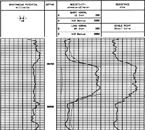
The diagram above expresses sectional View of an E-log – the SP-Curve, at the left side of the depth-track is in response to across-permeable-beds assuming that there are differences with the drilling-fluid as well as with the formation-water.
According to Meyer:
Along with permeability the SP also reacts to differences between the drilling fluid and formation water in ion type and salinity. The most common scale used for the SP is 5 millivolts (mV) per division or 50 mV across 10 divisions on standard API logging paper. The SP is used to identify changes in permeability, water salinity and dominant ion type (Meyer, 1998, p.56).
The 16-inches Normal (or the Short-Normal is it is otherwise regarded) takes measurement of the sphere-resistivity at almost a 3-feet diameter. The superficial evaluation curve would be subjective to the drilling-fluid which is made use for drilling the well. The Short-Normal responses are contrasted by means of a 64-inches Normal (otherwise referred to as a Long-Normal) based on the fact that the Long-Normal carries out the measurement of the sphere’s resistivity at almost 10ft by width; this tool conducts an intensified reading of resistance –an overwrap of the 2 turns on the readings is thus functional of the tool’s hole diameter, the bed’s thickness, as well as contrasting of the salinity that occurs within the drill-fluid and the water’s formation; Normal-curves have been made use of in the determination of lithology/water quality- at an instance whereby the e-log has been ran on sandstones or on solid rocks, the resistivity’s value become greater in region where there is added cemented concentration. However, this would be reduced at an instance where there is reduced cemented concentration or where there is the occurrence of a fracture. it is noted that, ‘the Normal Curves are run in the track to the right of the depth track, the 16-inch Normal is the solid curve and the 64-inch Normal is the dotted curve’ (Herbert et. al., 2008, p.104).
Equally, MacCallum et. al has identified that:
The Single Point Curve is mainly used to pick bed boundaries and for lithology; It is a linear measurement of resistance not a volume measurement, influenced more by hole-diameter and changes in borehole fluid than the Normals; The Single Point is run in the far right track (Hagiwara, 1996, p.3).
Guard Log
The Guard constitutes a deep-reading resistivity-tool which has been quite effective when used for thin-bed resolutions. Ordinarily, a Guard-Resistivity-Log runs in line with a Gamma-Ray-Log. The great metal-mass of this tool would not permit for any running of SPs in line with Guards –for this reason, the Gamma-Ray is a substitute. Meyer has noted that, ‘the Guard has bed resolution similar to the Single Point, but measures resistivity- it also has better bed resolution than the 16-inch Normal and sees deeper into the formation than the 64-inch Normal’ (Meyer, 1998, p.45).
One other benefit of making use of this is based on the fact that these curves do not reverse into thin-best as it is known of Normals. The Guard-Log could be run in either of fresh-water or in a saline-drill –fluid for measuring the formation’s resistivity value.
Thin-beds of average capacities possessing 2 Normals could be viewed as been existent on the Guard-Log. Based on the fact that guards are known to read when carrying out in-dept drillings into formations of resistivity-values, it is usual to observe Normals of up to 64inches in existing fresh-water-wells. A good illustration of this is an instance where the guard resistivity is within the ranges of 0 – 400 ohm-meter on measuring scales where as the Normals fall within the ranges of 0 – 200 ohm-meter and has a x10 backing scale that ranges within 0 -2000 ohm-meter (Meyer, 1998, p.45).
The Guard-Log has been created for oil-industry as a tool for salty-drilling-mud logging. The drilling-mud’s formation is such that it makes salty the formation-water and/or salty-water which is made use for drilling wells for the reduction of swellings available clay-formations.
Induction Log
The Induction-Log runs for the determination of formation-lithology in air-drilled holes/non-metallic cased-wells. It has 2 curves – a measuring Conductivity-Curve as well as a generated Resistivity-Curve. The running of a Gamma-Ray Log could equally represent an Induction Log because considering several monitored wells; the drilling is effected through methods that would not employ the usage of drilling-mud (rather, there could be only existing ground water as a lubricant). With the availability of the water in such wells, induction is achieved by measuring the conductivity/resistivity value in the entire well. Hagiwara found that the effectiveness of the log tool is based on the fact that it has, ‘a single transmitter, single receiver type with 19.7-inch spacing- the diameter is 1.4 inches, so it is small enough to log wells with 2-inch ID PVC casing- the tool is 64 inches long and weighs 4.9 pounds’ (Hagiwara, 1996, p.76). The development of the induction-type-log is aimed at easier mining in oil industries where there is a log-in of oil-based-drilling fluids which lack the ability of conducting deserved run-electric, guard-logs, as well as lateral (Hagiwara, 1996).
Lateral Log
Lateral-Logs are other deep-reading resistivity-curve, comparable to 64-inches Normal/Guard, which are made use of in lithology. The Lateral constitutes of 3 electrode-devices which have current-electrodes as well as 2 measuring-electrodes. The 6-foot-spacing corresponds to distances from current-electrode to measuring-point. Hagiwara, from his study has noted that, ‘The electrode configuration gives the lateral the advantage that it does not reverse in thin beds as the 64-inch Normal does and it develops out further in thinner beds’ (Hagiwara, 1996, p.98). One other merit of this has to do with its potential for measuring shell’s resistivity which constitutes formations of approximately 6ft off the reduction tools which are capable of influencing the borehole’s fluid. On the other hand, the demerit Includes the fact that produced curves lacks symmetrical composition as it is the case with 64inch normal and Guard- it is much more easier picking the lower parts of beds as compared to the tops. Equally, this constitutes a dead-zone which is located at approximately 5ft beneath bed-level.
(Hagiwara has included an example to include, ‘the bed just below 540 feet is not seen on the Lateral’ (Hagiwara, 1996, p.98). the illustration identifies advanced resistivity-values which are measured through the use of Lateral (otherwise regarded as dashed-curve). The advancement in the resistivity value is based on the fact that there is a lesser influence due to the borehole’s fluid as well as lesser bed-thickness effects. Hagiwara equally noted that, ‘the sand at 520-530 feet cannot be seen as well on the 64-inch Normal because of the bed thickness’ (Hagiwara, 1996, p.98). When the beds have an increment in thickness, there will be a correspondence in the 64inch-curve. This behavior, however, is lacking in the lateral- it lacks the capacity of responding in the same way to the bed-thickness.
Next Generation LWD Tools and Processing Improve Resistivity Accuracy in High-Angle and Horizontal Wells
Proper evaluation of propagation-resistivity logs could constitute quite taxing experiences, particularly when high-angled wells are considered. Based on the fact that LWD propagation-resistivity tools function at high frequencies, effects from logging-environment could appear rather severe particularly when considering the tools instead of induction and laterolog-tools. At instances whereby the resistivity-log curves are separated, there could be an assumption that the outcome of a unit cause such as invasion. Based on factual happenings, there is the likelihood of having influenced logs from multiple effects. Hence, the fundamental tool for an appropriate evaluation of logs could be based on the identification and differentiation of the several effects of the environment. With a proper knowledge of involved effects, there could be an equal response in terms of correcting data which could be utilized for accurately evaluating the logs.
In his discussions on resistivity tools, Hagiwara noted that, ‘Today’s new generation LWD propagation resistivity tools record more measurements than earlier systems, making much more accurate formation evaluation possible’ (Hagiwara, 1996, p.78). Based on the capability of present-day tools to be used for recording more resistivity-measurements, it is more possible to arrive at more reliable information concerning the statue of boreholes. Particularly, present-day tools are reliable towards analyzing data on high angled or horizontal wells which ordinarily could present some difficulty, especially in the identification and differentiation of environmental effects. Hagiwara has noted that, ‘the effects differ between horizontal and vertical wells’ (Hagiwara, 1996, p.97). Equally, it has been resolved that, ‘in vertical wells, environmental effects include shoulder beds, dielectric constant, and invasion’ (Hagiwara, 1996, p.97). The situation with horizontal wells present complicated handling of effects such as, ‘eccentricity, bed boundaries, dielectric anisotropy (εv, εh), resistivity anisotropy (Rv, Rh), and asymmetrical invasion’ (Hagiwara, 1996, p.78).
In present days, there is remarkable advancement in the rate at which data is been processed through the use of software that incorporates the combination of present-day tools and multiple measurements which are used in identifying and correcting emergent effects. When corrections are effected, the used software would then produce resolutions that would correspond with the resistivity-curves such that, ‘fixed radial depths of investigation at 10 minutes, 20 minutes, 35 minutes, and 60 minutes’ (Zhipeng et. al., 2007, p. 29). From studies conducted by Herbert et. al., (2008), it was noted that, ‘field comparisons to wireline array resistivity measurements demonstrate the robustness of the method under a variety of formation resistivity environments and clearly show where interpretation methodology is improved’ (Herbert et. al., 2008, p.109). A clear effect from this that comes from a considered environment which the study has failed to address is eccentricity. Good enough, eccentricity could only be considered as been problematic at instances whereby there is the existence of voluminous contrasts of the formation-resistivity and the mud-resistivity, or when bigger boreholes are been considered.
Even though used techniques for interpreting the methodologies may be instrumented with the use of Baker-Hughes-INTEQ’s MPR tools, their application may be boundless when it comes to multiple-investigation-depths. Herbert et. al noted that, ‘the MPR operates at two frequencies [2 MHz and 400 kHz] and two spacings [23” and 35”] (Herbert et. al., 2008, p.49). Equally, Herbert et. al., (2008), from studies conducted noted that, ‘Phase difference and attenuation resistivities are measured at each frequency and spacing, for a total of eight compensated and borehole-corrected resistivities’ (Herbert et. al., 2008, p.51). Further, Herbert et. al., (2008) noted that, ‘a combination of both raw phases and compensated resistivities is used to generate the four, fixed-depth curves, facilitating improved log interpretation in high angle and/or horizontal wells’ (Herbert et. al., 2008, p.78).
Processing and Interpretation Methodology in Vertical and Low-Angle Holes
There is the establishment and definition of processing-methodology for low-angled and/or vertical wells (Hagiwara, 1996). The technique makes use of eight raw-phases and/or eight-compensated resistivities for the generation of resolution matches, four-curve, and fixed-depths of investigative presentations which are comparable in terms appearances to modern multiarray wireline induction-tools. This is because:
- This low angle method corrects the resistivities for shoulder bed effect via a deconvolution routine and dielectric constant using a Complex Refractive Index Model (CRIM); and
- Fixed depths of investigation are significant for propagation resistivity logs because the investigation depth of phase difference and attenuation resistivities that are heavily dependent on formation resistivity, making it difficult to accurately estimate invasion depth at any given resistivity without using radial response models (Meyer, 1998, p.5).
Processing and Interpretation Methodology in High-Angle and Horizontal Wells
Based on the fact that the environment is capable of influencing and causing changes in line with increments in relative-dip angles, this reflects the processing methodology equally. Meyer noted that low-angle processing would the work only at instances where the relative-angles are below 65° because there is a limitation of deconvolution-routine at this point. Meyer noted that, ‘this routine therefore must be removed from the processing scheme’ (Meyer, 1998, p.17). More so, when horizontal wells are taken into consideration, shoulder-bed-effects become greatly substituted by bed-boundary-effects and/or influences of under-beds. Meyer further noted that, ‘the effect is greatest on deeper reading measurements [especially where there are large resistivity contrasts between the bed that the tool is in and the adjacent bed] (Meyer, 1998, p.16). The effects are not easily accounted for because of their heavy reliance on formation-resistivity as well as on resistivity-contrasts that occur at bed-boundaries.
One other effect that needs to be corrected when considering high-angle wells is resistivity-anisotropy. According to Meyer, ‘the effects of anisotropy on propagation resistivity logs have been well documented in the literature’ (Meyer, 1998, p.16). But even with so much information on Anisotropy, there has been a correction complexity as regarding propagating anisotropic resistivity-logs through demonstrations that identify with solving anisotropic challenges- especially, through the use of non-uniqueness; this happens particularly when there is a single space.
To enable addressing the issue at hand, the highly angled processor schemes first make corrections for bed-boundary effects that make use of a quantitative-geosteering technique that comprises inversions to a 2 layer-model (Meyer, 1998). When such an instance is considered, the unknown shoulder-bed resistivity, the MWD-tool – bed distance, as well as the horizontal/vertical bed resistivity becomes non determinant. The bed-distance inversion then would be conducted based on point basis instead of on the larger filtering-operations known with majority deconvolutions as emphasized:
- After bed boundary effects are removed, a second inversion simultaneously calculates a best fit solution for dielectric constant at each frequency, anisotropy, and invasion. These effects are best inverted together since any one of them will be miscalculated if inverted alone; and
- Furthermore, the miscalculation of one of these parameters would invariably lead to the miscalculation of the others (Hagiwara, 1996). The last step in the processing routine transforms the corrected data into apparent resistivity values at fixed radial depths of investigation (Herbert et. al., 2008, p.24).
Multi-Parameter Propagation Resistivity Interpretation
Modern induction-tools have been made in such a way that there is the possibility to have them routinely developed for the production of curves at fixed investigative-depths. But the steps which could be followed are not quite extendable to multi-array Measurement-While-Drilling (MWD) resistivity-tools even with possible current-tools making adequate measurements based on the fact that aim of utilizing the MWD initially was for the creation of fixed-depth-curves which may be compared in all standards with present-day wireline information carriers. sadly however, emergent challenges that were based on high-dip-angles, unexpected dielectric-constant, eccentricity, anisotropy, as well as on a number of differing occurrences were noted to get worse when the system was subjected to 2MHz rather than when it was induced at a reduced frequency. Equally, the MPRTM system produces thirty two varying measurements with the use of 4 transmitting units, 2 receiving units, as well as 2 of 400 kHz and 2 MHz frequency monitoring units. The 2 receiving units are positioned in such a way that they are at the center of the 4 transmitting units. there could be a combination of the 2 transmitting units with 2 receiving units in order to develop short spaced arrays, where as the 2 external transmitting units could be made use of in terms of long-spacing the arrays. The system also comprises of 4 varying transmitter-receiving produced arrays, including a two MHz long-spaced (35inches) unit, a two MHz short-spaced (23inch) unit, as well as another set of 400 kHz frequency units. The various arrays, together, produce 2 completely compensated measurements (each of the produced measurements come from the various attenuations) – in all, these amount to 8 measurements.
Further, the MPRTM is effective in terms of producing unaltered measurements through the use of a singular transmitter as well as through the use of a receiving unit. Even though, the measurements carried out have a positive statue based on the fact that they are shallow, there are also negative aspects whereby there could be poor calibrations. consequently, the measurements have to as a matter of necessity be calibrated through an artificial means- this is done by putting them side by side with a completely compensated measurement (ordinarily the two MHz long-long-phased unit is preferred). It has been noted from studies that:
The raw phases are the shallowest and most accurate of the raw measurements, and eight of them are used in the computation of the fixed depth curves. These eight curves are added to the eight fully compensated curves to yield 16 different measurements (Herbert et. al., 2008, p.29).
Wireline Comparison
A log structured with the use of a 6(3/4) inch MPRTM was shown to be effective in a 9(7/8) inched borehole. The resistivity of this mud constituted of 0.25-ohmmeters, thus enabling the possibility for an invasion which would be conducted as relating the resistivity of relocate fluids through actualization of higher-resistivity-zones whereby there would occur tight-streaks, and well the neither of the zonal intervals may be taken into consideration as a pay-zone. Expectedly, the produced curves could equally overlay and express the possibility of the absence of invasions thereby depicting non-inversion of the compensated information which may be used for re-logging of the interval which were earlier considered. The attenuated resistivity curve (identified by an investigative depth as well as a poor vertical resolution) was produced at less complicated shades. These 8 curves were separable through a majority of the logs, and this created a lot of difficulty particularly in terms of determining invasive zones. In any case, the invasion of the information which was gathered using the same intervals showed the occurrence of basic invasions merely in the considered zone occurring at 120-160 ft. quite a number of slight invasions equally expressed tendencies of occurring at the location at the heights of 70-85 ft as well as from 195ft up to where the graph’s plot stopped.
Reference List
Anderson, et al., 1990. Response of 2 MHz LWD resistivity and wireline induction tools in dipping beds and laminated formations. SPWLA Annual Logging Symposium, 23 (7), p.8.
Barnett, W. C. and Meyer, W. H., 1991. Radial Response of a 2 MHz MWD Propagation Resistivity Sensor. Texas: SPE Annual Technical.
Bittar, M. and Rodney, P., 1996. The effects of rock anisotropy on MWD electromagnetic wave resistivity sensors. The Log Analyst, 12 (4), p.27.
Hagiwara, T., 1996. A new method to determine horizontal resistivity in anisotropic formations without prior knowledge of relative dip. SPWLA Annual Logging Symposium, 16 (19), p.24.
Herbert et. al., 2008. Identification of Formation Fluids Using the Dielectric Constant Determined from LWD Wave Propagation Measurements. SPWLA 49th Annual Logging Symposium, 2008.
MacCallum, et. al., 1998. Determination and Application of Formation Anisotropy Using Multiple Frequency, Multiple Spacing Propagation Resistivity Tool from a Horizontal Well. SPWLA Annual Logging Symposium, 17 (9), p.23.
Meyer, et al., 1997. Multi-parameter propagation resistivity logging. SPWLA Annual Logging Symposium, 45 (16), pp.46-49.
Meyer, et.al., 1994. A new slimhole multiple propagation resistivity tool. Annual Logging Symposium, 12 (8), pp.18-25.
Meyer, W. H., 1998. Interpretation of propagation resistivity logs in high angle wells. SPWLA Annual Logging Symposium, 62 (3), pp.2-3.
Roberts, et al., 2007. The Employment of Resistivity Modeling to Elucidate and Explain Complex LWD Resistivity Responses in Mumbai High Field. SPWLA Indian Regional Symposium, 8 (3), p.2.
Wu, J.Q. and Wisler, M. M., 1990. Effect of Eccentering MWD Tools on Electromagnetic Resistivity Measurements. SBWLA Annual Logging Symposium, 45 (3), pp.86-87.
Zhipeng et.al., 2007. Joint Inversion of Density and Resistivity Logs for the Improved Petrophysical Assessment of Thinly-Bedded Clastic Rock Formations. SPWLA Annual Logging Symposium, 7 (3), p.57-61.