Abstract
Natural resources are a gift of God to mankind. Natural resources play a pivotal role in the success of any nation. Gas and oil reservoirs are different and this report deals with numerous approaches in order to Predict Reservoir Performance of a Natural Gas Reservoir. There are a number of approaches that helps in obtaining optimum level gas production. The later section of this report deals with the use of the artificial neural network in order to obtain optimum gas production.
Introduction
For a success of any nation, it is very important to use all natural resources at their optimum level. Natural resources help a lot in gaining success. This is a technology era, and most of the work is done by the machines for saving time and money. Machines are beneficial in every aspect but they cannot replace human resource. Natural gas is one of the most important resources consisting of methane. A large number of countries are using their natural resources in order to achieve high goals in the market. Natural gas has several uses few of them are as follows: Power Generation, Residential domestic use, Natural gas vehicles, Fertilizers, Aviation, and Hydrogen. Natural; gas is also used in the manufacturing of glass, steel, plastic and paints etc.
Natural gas is widely used in trade as a commodity in Europe, United States of America and in Netherlands. Rest of the world is also using natural gas as a main resource in order to achieve high objectives in market. There are number of forms of gas used by several countries. Compressed natural gas is also widely used worldwide for different objectives. Canada is a large producer of natural gas and CNG is widely used in Canada as an economical motor fuel.
In United States of America, the CNG is also used at economical rates by number of consumers. CNG is widely used in local cities and country fleets. In Canada and other parts of the world, CNG is also used for public transport. Italy has a largest number of CNG automobiles in the world. Canada is the fourth country in the world for CNG automobiles use. They have a huge number of automobiles at their place. The increase in CNG automobiles is due to the increase in prices of other fuels. CNG is an economical fuel for automobiles as well as for public transport. Argentina and Brazil are the two countries which have largest fleets of CNG vehicles. Argentina and Brazil have 3 million vehicles by the year of 2008. In Asia, CNG is one of an economical fuel for all automobiles. In Asia, CNG costs 18.90 PKR.
There are many countries using natural gas vehicle that uses compressed natural gas or some vehicle also uses liquefied natural gas as a best alternative to other automobiles fuel. There are number of advantages of natural gas as it is economical, it is widely used as an automobile fuel. Despite its advantages some limitations are also attached with the natural gas which includes fuel storage, distribution at gasoline fueling stations. Fair Natural gas distribution is quiet difficult at a number of fuel stations. Oil and natural gas were usually reformed from the extracts of prehistoric plant and different animals.
Millions of years ago, oil and gas were found in the source rock deep within the earth through tiny, connected pores and spaces in the rock. Gas Reservoirs are usually located 100 feets below the earth. In United States, natural gas reservoirs are usually located 1000 feets below the surface. A number of reservoirs contain oil, gas and water. They are usually separated on the basis of density gas being on top, then oil and then water. With the aid of technological innovation it could be possible to retrieve more reservoirs for instance; new drizzling techniques have made it so easier to retrieve more reservoirs with limited resources.
Technology advances have made it so feasible to extract oil and gas reservoirs horizontally instead of vertically. Horizontal retrieval made it so easy to extract a large amount of reservoirs within limited resources. Advance resources have enhanced gas industry ability to find finite amount of oil and gas created millions of years ago.
Background
The main objective of following study was to figure out the various phenomena and pressure behavior at gas field.
Natural Gas Field Development
Oil and natural reservoirs are produced with the aid of following anaerobic decay of organic matter deep under the surface. Oil and gas usually found together. In common usage, normal deposits usually rich in oil are known as oil fields, and deposits rich in gas are known as gas fields. Global demand of gas is growing day by day and now gas has become an essential element for most of the industries.
Demand of gas is increasing continually comparatively to any other fuel. Natural gas demand in long term will highly depend on numerous factors i.e. consumers needs and commercial needs, restriction of electric and natural gas industry, population and demographics centers, energy efficient regulations, transportation needs, environmental emission regulations, efficient equipment and processes, manufacturing of new good with less input. Fortunately, a natural gas is not limited in supply. According to the current estimates, there are approximately 5,500 trillion cubic feet of proven gas reserves.
Nowadays, United States and Western Europe, one of the largest natural gas consumers is on the decline path. The declining output is being supplanted by new developments and productions is different regions of the world i.e. Africa, Middle East, Latin America. The transportation of natural gas over long distances is a major challenge in order to keep market supplied needs new development methods and techniques in production. In recent days, there is an adjuring need to extend life of major field and extensively access reserves that were once declared as so expensive to exploit (Poettman 302).
There is a special need to enhance expertise and services in order to minimize risk, maximizing reservoir deliverability, reducing time and cost by applying effective measures and to enhance ways to deliver technical innovations in order to use maximum resources. Strong measures are required in field development in order to increase the recovery from natural gas resources.
All natural resources require special environment, some safety precautions for effective production and uses. There are some gases reservoirs exist which contain high levels of hydrogen sulfide which requires highly trained technical staff and respirators so that risk could be minimized. Different gases found in natural gas reservoirs i.e. corrosive or reactive gases highly influence downstream facility equipments and safe operations.
A natural gas resource, reservoirs understanding is quiet complex and requires special attention in order to manage hazards and ensuring safe operations under limited time. Quality is one of the important factors involved in all domains. Quality speaks itself when ever quality is best, it works itself. In order to make changes and improvement in gas field it is necessary to take preventing measures for reducing risk. The focus on quality standards helps a lot in reducing risk factors and cost factors. Quality can be improved by understanding the needs and requirements of costumers and the technology development in order to meet requirements.
Service quality can be improved by using different Real time survivor solution by which an entire team is connected via satellite and all team members can see the production process, production data, which helps in making quick decision both in short as well as in long run. The basic goal of using different production methods is to obtain maximum recovery of amount of reserves per well bore. Using new and advance production methods accomplish the following:
- Improve Reservoir understanding: New and advance production methods help in improving reservoir understating through landmark rapid prospect generation and Westport technology center analytical services.
- Superior identification of intervals: Using drilling and Formulation evaluation division provide superior identification of commercial intervals.
- Enhance Recovery of Reserves: They enhance access recovery of reserves with the aid of state of the art technologies such as Smart well, completion’s technology and fiber optic technology.
- Minimization of Formation Damage: They help in minimizing the formation damage and also enhance productivity with synthetic-based fluid and unique N-flow beaker technology for cleaning drills. The core drill-N provides a right choice for successful completion of higher temperature systems.
- Real time reservoir characterization: They enhance in delivering Real time reservoir characterization by using Real time Reservoirs Evaluation (RTRE) in low pressure reservoirs. They enable the identification of new producing intervals within a zone. It also allows the increased production in combination with under balanced Applications Technology.
- Maximum Hydrocarbon Production: the main goal of using new and advance technology is to maximize the amount of hydrocarbon by minimizing total recovery and increase initial production.
Following solutions help in the production of Maximum hydrocarbon.
- Total system development Approach: Total system development approach originates with the original design engineering cycles through execution and feedback of continuous development improvements. There are many processes have improved the recovery from many gas fields dramatically.
- Acquiring early and accurate formation measurements: Different technologies and instruments help in acquiring early and authentic measurement formation with the aid of compensated thermal neutron sensor.
- TI logging technique: Ti logging technique that needs high quality data including total porosity, free fluid and bound volumes and permeability estimates.
- Non productive time reduction: Time is one of the most important factors in overall production and field development. Results achieved in les time are always considerable as an excellent achievement. Hydraulics modeling software and real time drilling simulator is widely used for improved holes cleaning, swap pressure and ECD values.
- Encore System: Drilling deep holes has been an important aspect in gas development. Encore system is widely sued in drilling deep holes efficiently. Bariod’s olefin based system also helps in drilling deep and hot gas wells.
- Deeper and higher pressure wells: The use of Depth star safety valve system which is now considered as a new bench mark in completing deeper and higher pressure wells. There are number of other technologies which also help in the same vein.
- Perforating Performance: Perfpro system is widely used in order to improve perforation performance up to 12% in Shells’ penguin field.
- Hydraulic Fractures in multi layered reservoirs: Only use of advance technologies can help in obtaining increased level of gas and other reservoirs.
- Reduced cycle Time: Time and cost are the two most important factors in production of reservoirs. Degree of production can only be identified with the aid of these two factors. Cycle time can be reduced by using any of the advanced technology like FM 3000 series bits, CUDA reamers, GEO tap formation pressure tester and other technologies.
- Conductivity stimulation technology: Proper use of technology and software plays a pivotal role in the production of gas and other reservoirs. They enhance the capability of retrieving reservoirs. Conductivity stimulation technology is widely used in order to extend the productive life of gas reservoirs. Conventional fracturing methods are also used in order to increase capability of production.
- Water management solutions: Water management solutions are one of the major challenges faced by operators. Following two innovations have proven their values in gas production field.
- Water Web service
- Quick look simulator
Water web service is widely used in order to reduce the ability of water to flow through the formation matrix without any restriction with hydrocarbon.
Special Services
There are number of special services available which are specially designed in order to reduce time and cost cycle in gas production field. High pressure and high temperature services are specially designed in order to maximize reliability and mitigate risk with the assurance of safety and environmental protection. CBM (coal bed methane technologies) offer an excellent life cycle management which involves numerous technologies for CBM optimization.
Need of intervention and re drill
Few days ago, operators were facing the major challenge of maximize intervention and re drill problems in critical wells. They want solution which must ensure the deliverability for the lifetime of their high rate at critical places. Gas migration vents that usually occur during the life of a well can seriously conquer operator’s ability for the production of gas from the reservoir efficiently. Such situations are extremely to repair as they need special attention, cost and time. They also play part in lost production. There are a number of software’s and technologies available in order to solve this problem.
New and advance technologies also give complete ease to operators by minimizing cost and time of overall production. There are number of factors involved in the production of gas which need a dramatic change in order to produce optimum level of gas from reservoir. Reduced time and cost proves successful achievements in the field.
Predicting Reservoir Performance
Reservoir performance in gas field is considered as one of the growing field in the market. Predicting gas reservoir behaviors’ main objective is to develop a flow rate versus time relationship from initial point to final point. Considering only reservoir, following procedure is proposed:
- Select any value from pressure decline curve in order to determine the quantity of cumulative gas produced. In order to increase accuracy, use small pressure increments.
- At the selected reservoir pressure obtain open flow potential from the deliverability curve. Flow potential is usually based on Pwf=0 and thus it is variable of maximum potential but it’s not like to be a flow rate. Fix allowable producing rate as one-fourth of the flow potential. If on selected point: producing rate (qc) < allowable producing rate (qOFP/4) occurs then use contract rate for time interval.
- Time required in order to produce gas is as follows:
T=Gp(over interval)/q(allaowable)
- Now repeat the step with lower values of gas reservoir until high peak is reached. In this step production rate and cumulative production vs time would be identified.
- The duration of overall period can be calculated with the aid of following formula: tc=Gp/Qc. For the remaining time it is highly recommended to divide rate interval in to equal parts in order to calculate the cumulative production for each. The time required to produce the gas is followed by
Inflow Performance Relation
In 1968, Vogel established a strong relationship for flow rate prediction of a solution gas reservoir in terms of well bore pressure which is highly based on reservoir simulation estimates. The development for an analytical result for the solution is usually written as follows:
According to above equation, analytical results for the solution can be calculated with the aid of above formula (Camacho 58). The main problem occur in such case is the issue of the reliable permeability) and the connection of effective/relative permeability on saturation point which usually requires that the saturation distribution must be estimated. Another logical step was to correlative the flow rate-pressure behavior for the phase liquid or gas case with the aid of pseudosteady-state flow model. For an alternative solution gas-drive reservoir the pseudosteady-state flow model is used in many cases (Velázquez, 2007).
Pseudo-steady state equation
The generalized Pseudo-steady state equation is highly depends on number of different parameters. The Pseudo-steady state equation based on average reservoir pressure for a well area in the equation Sm represent mechanical represent factor because of drilling and completion related well damage. S, the skin factor s is the addition of skin factors due to perforations and acid simulations.
There are numerous approaches available in order to predict reservoir performance but pseudo state equation is one of the best equations used for predicting gas reservoir.
Planning Optimum Production
Gas and oil productions are not same, there is usually a misconception occur that oil and gas reserves are same but there is a need to identify the difference in oil and gas reserves. Oil and gas reserves and production is different not just because of different physical characteristics and properties but they are also different purely for economic reasons. Optimum level oil field production is possible by applying different techniques but optimum gas production is directly linked with market via pipeline.
Therefore the reservoir behavior doesn’t always help in determining the best depletion pattern as there is a strong restriction that market must accept provided level of gas. In a gas field, there is a strong bond and relationship exists between the production and marketing phases of the gas. In the gas field, some restrictions are always involved and production could not be started until the gas sales contract has been signed. There are few basic parameters which are required to be determined before the development has begun. Determining these parameters is not possible in case of oil production as oil doesn’t pose a direct link with the market.
The detailed knowledge of these parameters in the oil field and in the planning of gas field development pattern in linked with gas sales signed document is at risk to many uncertainties. In later sections of this paper various steps have been simplified in order to avoid undue complications in gas development field. As, it is stated above, that there is a vast difference between gas and oil reservoirs due to economic reasons. In case of oil reservoirs water drive usually have a high recovery factors than depletion type fields. In case of gas reservoir this process becomes reverse. The reason of this effect is water doesn’t displace all the gas in gas reservoir.
An appreciable amount of gas is usually trapped by capillary forces in the spaces of the rock and is by-passed. This gas is usually termed as residual gas and expressed in percentage as 40 percent to 20 percent. IF the water drive decreases in the strength in result of which ultimate recovery will be higher and the same case will occur with a weak water drive, ultimate recovery in weak water drive may be little higher in case of depletion pattern. Water drive strength is highly depends on three factors which are listed below:
- Permeability of formation
- Strength of water drive
- Time Factor
- Permeability of formation is an ability to allow fluid to pass through vessels. Usually, formations with high permeability, the flow of gas is quiet easy and it takes place with low pressure drops. Consequently formation with low permeability even with high pressure drops results in low flow rates of gas. The same results will occur for water, low permeability, the less chance of water drive occurring.
Strength of water drive
Strength of water drive highly depends on the size of reservoir the larger the size of reservoir the weaker the water drive occurs.
Formation of Gas
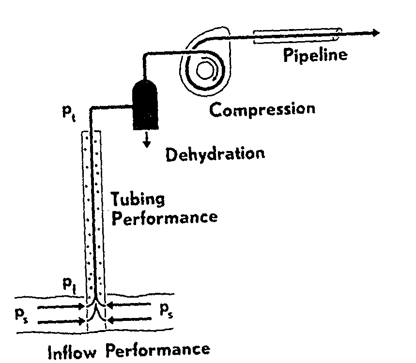
Now lets be practical and see how much gas can be produced from one well and how do we produce it. To actually understand it there are several tests that are done and performed. Every second test is reliant on the previous test. One very important thing that we should know is that the gas collected in the reservoir must flow properly through the well. The gas then flows in the upward direction. Two very common things are experienced during this test, first thing being friction loss and dropping down of pressure and second thing the amount of water present. Even if the production rate of gas is very fast but still the accumulation of water will take time.
This results in the increasing density of gas. In the end the gas would be dehydrated and ready to deliver. The important stages of the formation of gas include the static pressure of well being measured, then production of gas at various rates and last but not the least the dropping down of pressure. After this, the well has to be closed to see whether the pressure will build up again or not. If it does not happen it actually means that the reservoir is too small for the production of gas.
Coming on inflow performance, we must know that a line is drawn from one point to another and this is actually known as the inflow performance relationship (Ikoku, 1992). The production rate of gas that is obtained at the maximum value is called open flow performance. The maximum production rate is usually less than the open flow production that is obtained by the unbroken curve.
Explaining the Difference
The flow of gas obeys the Darcy’s law, which is this that the coming down of pressure on the given distance is comparative to the flow rate of the fluid considered. This may be the case for oil but it not always works out in the case of gas. This happens because this law neglects the forces of inertia. According to Darcy’s Law, the thickness of gas in the reservoir is 1/50 of light oil. Considering all this we can say that the gas flow speed is 5o times higher than that of oil flow. With inertia effect the density of oil is higher than that of gas. Now it is clear that the mass flow effect in gas field is actually more imperative than in oil fields.
Time also plays a very important role in the production of gas. Let’s say if the production period is 3 hours, then the pressure drop would not be circulated all through the reservoir. The gas that will be produced in only 3 hours is that which comes from that part of reservoir that is closer to the well bore. If we give it more time the gas will be produced from other areas as well. So if the gas production period is increased then the result would not be that good. So the 3 hours inflow performance is very important in order to get the favorable results. The 3 hour inflow performance is commonly known as “stabilized inflow performance”.
Let’s now understand how gas field is developed. In some parts of the world the wells are not spaced over the reservoir but are actually clustered jointly. Another very famous way of developing this kind of gas field would be by drilling well in vertical position. Today the gas field development is a common practice especially when awl in deep water. It is very simple to drill two wells close to each other but there is some problem in that. This problem is that the close construction of wells can end up in mutual well interference.
The high permeability formation of wells actually has closer wells and opposite is the case with low permeability formation of wells. Both the cases are different from each other in many ways. There are many formulae derived to make the approximation of the intervention between the wells in a bunch.
Vertical Flow Performance
The vertical flow performance of gas is known as tubing performance. The well flowing pressure is different from tubing head pressure. Say we have two different types of tubing, one is 3 inch and the other is 5 inch, the production rate of 5 inch tubing is larger than the 3 inch tubing.
Well Performance
The intersection of inflow performance curve and tubing performance curve figures out the well production rate at the following conditions:
- Static Reservoir pressure
- Type of well inflow performance
- Tubing size
- Tubing head pressure
The loss that is acquired by the stabilized inflow performance with respect to 3 hour test inflow performance will be remunerated by the raise because of the larger tubing size. Lowering the design production rate for a high productivity well will barely outcome in any major rescheduling of compressor setting up, and for low productivity well, lower well potential can have an important effect. This should be done by the reservoir engineer who designs the entire task for future. This is not only a technical point but economical also.
Gas Field Production
Following are the different types of patterns for the development of gas field.
Off take Pattern
This pattern is limited by two constraints. The market should be able to absorb the gas in this pattern. This actually affects the production rate of gas. In this pattern the total amount of capital expenditure required depends only on the level of production.
Basic Production Pattern
In this pattern the economic result of future gas production is estimated on the basis of the field of production in which no further drilling takes place. The more the wells are drilled the production rate will increase. The total rate of production is actually calculated by multiplying the number of wells and highest production rate per well. The future life of any gas filed can be mathematically represented in the following way:
Optimum Off take Patterns
In order to understand this we must first know what optimization is. Optimization is the optimum production rate of a gas field reached by the increase in the production rate by increasing the mount of wells that no longer supply to an increase in present value profit. It is clear that the production rate depends on the values of parameters alpha, beta and gamma which are given in the following figure.

Example
The highest graph shows the optimum growth pattern for a field having a large part of reserves which can be formed before the setting up of compressor is necessary. The perfect example of optimum offtake pattern is given below in the form of diagram.
At the end we can only say that a gas field is closely related to the gas market and whatever optimum off take pattern from field point of view are not always best. It is the reservoir engineer who has the biggest responsibility of indicating the range of optimum patterns.
Artificial Neural Networks
Neural network is usually referred as a circuit of biological neurons. Artificial neural network is composed of artificial neurons or nodes. Artificial neural network has two prominent uses:
- Biological neural networks
- Artificial neural network.
Biological neural network are composed of biological neurons and are functionally linked with the peripheral nervous system or central nervous system. Biological neural systems are widely used neuron science field. Biological neural network performs specific physiological functions in laboratory.
Artificial neural network: Artificial neural network is a group or collection of artificial neurons. Artificial neural network is widely used in order to gain understanding of biological network. Artificial neural network is also used for solving artificial network problems without creating real biological model (Van Dam, 1967). Real biological nervous system is very complex and sometimes needs to be solved via artificial neural network techniques. Neural network is widely used in a number of applications where the complexity of data makes the structure little complex by hand practical. Neural network is widely used in following real life applications:
- Function approximation, or regression analysis which includes time series prediction and data modeling.
- Classification, sequence recognition, novelty detection including pattern and sequential decision making.
- Data processing, including blind signal separation, clustering, filtering and compression.
Famous neural network soft wares are the GBLearn2 library of the Lush programming language, Wolfram Research Neural Network package which structure is based on the Mathematica computing environment; the Math Works Neural Network Toolbox which is based on the MATLAB computing environment; the AMORE and neural packages of the R programming language etc. the study of neural network in order to predict performance of complex structures (Harstad 34). The study of near critical gas reservoirs has been a rich area of research during past few decades. Gas reservoir usually poses singular depletion behavior.
Singular depletion behavior differentiates gas reservoirs from other reservoirs. Generally tapping gas recoveries without heavy pressure maintenance generates high surface gas recoveries with the combination of relatively low condensate recoveries. Existence of a hydrocarbon liquid module upon depletion is typical to other similar systems, and few concerns are involved in it but major concerns are linked to the loss of valuable fraction of heavier hydrocarbons and the linked impairment in gas development and production from the wellbore region. In order To facilitate reservoir pressure support, the participation of surface gas for instance, nitrogen. Nitrogen is widely known for the perfect pressure maintenance. Pressure maintenance can be easily identified by keeping the reservoir pressure above to dew degree.
The function of the gas injection operation is to fixed gas condensate reservoir in order to bind to the flow characteristics of phase behavior of the fluid. Implementation of artificial neural network (ANN) technology is very beneficial in order to optimize production of gas against the establishment of a capable system learning in order to understand relationships between the input and output parameter to judge the response of compositional gas simulation of the overall operations in gas reservoirs (Nabil, 2007).
A number of Parametric studies have been conducted in order to find out the most authoritative reservoir for establishment of maximum protocols production, for the deployment of the pressure maintenance operation. In result, an excellent tool pressure maintenance implements operations in gas condensate reservoirs is developed. With the aid of resultant tool a fast, reliable, and inexpensive results can be determined using the proposed approach while captivating the important flow and thermodynamic properties built in to systems without recurring to descriptive and expensive studies.
There are numerous artificial techniques which can be used in order to solve numerous gas development problems. If a problem can be solved using simple conventional techniques than no body would like to use neural network technologies. In some cases, where conventional techniques fail than individuals usually go for neural network techniques in order to solve complex problems. For example, maintain a checkbook is not recommended using neural network.
Polynomials and different equations are always used in order to solve simple problems. Neural networks have proven great potential for obtaining accurate analysis and results from previous large databases. Neural network is widely used in such cases where conventional methods fail. This generally happens when all parameters are not known. Neural network are widely used to predict or virtually measure formation including porosity, permeability and fluid saturation from conventional well logs.
Using well logs as input parameter with core analysis of the corresponding depth, these characters usually help in predicting heterogeneous formation. The application of neural network in gas and petroleum industry is increasing daily after major changes in ANN design (Nabil 67). ANN modeling is widely used for the development of a model for the prediction of water saturation. A normal methodology was built in order to cover various design issues in the proposed ANN modeling.
The workflow model proposed the solution to how the neural network can be translated in terms of enquiring the contribution of input variables and comparing the obtained output with other available regression models. In addition, the workflow usually emphasizes on the data relevancy and the importance of identifying the unceasingly in the input data before using it in the model.
ANN proposed three layered feed-forward neural network model with various hidden neurons. Multiple neural network model approach is one of the best novel approaches which combines a group of neural network with each provided component in neural network in order to predicting a different time period. The approach is specially designed to enhance the accuracy of predictions.
Problem statement
Oil and gas are the two biggest natural resources available in many parts of the world. There is a big difference between oil and gas reservoirs and both reservoirs play an important role in economy of any country. Oil and gas production optimization have been a need of all countries. A number of petroleum engineers covered optimization of a gas and oil production for several years. Predicting gas reservoir performance is an essential part foe the development in the gas field. Without predicting gas reservoirs, it is not possible to increase gas production by any means. Optimum development plan play pivotal role in gas development domain. The ODP highly depends on properties of reservoir and market to be served by the field.
There are three main factors which affects natural gas production. The three factors are as follows:
- The reservoir
- The well tubing
- The surface network
Economic consideration also affects a lot in the gas development and maximizing gas production.
Inflow Performance
Methodology
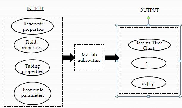
Gas production reservoirs are an important aspect for optimization of gas production. Methodology of gas performance is divided in three parts: input, Matlab subroutine and output.
Inflow performance relationship is a linkage between flow rate, q and pressure down. Lets take an example of 2 wells with dry gas reservoir and poses following attributes:
Tubing system: According to tubing method, performance prediction is based on
The main objective of this plan is the production of two wells at the maximum rate of 3.12 mmscfd until such a time when the reservoir pressure has declined to a point where this rate can no longer be sustained.
The objective is to predict reservoir performance of the field beginning at t = 2 years and lasting until abandonment, estimated to be qa ~ 300 mscfd. The performance prediction chart is shown below:
Now if we talk about the constant rate period then there are five steps in total that should be kept in mind. Firstly, one must use the Cullender & Smith Correlation method to find out the lowest bottom hole pressure, which will maintain a flow rate of 3.12 mmscfd per well calculated against the wellhead pressure.
Secondly, calculate matching Pr from pseudo-steady condition equation for radial course of real gases at low pressures. In view of the fact that µ and z-factor are pressure reliant, this process is done by an iterative method and started by presumptuous a Pr between Pi and Pwf. Here is the formula: Pr2 = pwf2 + 1422[ln( – 0.75 + s’]
Thirdly, compute equivalent value of increasing gas using material balance equation for Gp.
- Gp =G[]
- Gp = 7.73 Bscf
Fourthly, estimate gas formed for the duration of steady rate time period.
- Gp(constant rate) = Gp – Gp(buildup) = 3.81 Bscf
Lastly, determine predictable time period to make these reserves.
- t = 610 days or 1.67 years
Now let’s just study how to decline the rate period. The values and equations used above would be used in this prediction process as well.
Firstly, reduce pressure by an unspecified value. Here, 100 psia is used.
- New Pr = 795 psia
Secondly, find out z factor and compute p/z at this pressure
- z = 0.935, p/z = 850 psia
Thirdly, bring up to date increasing gas generated for new Pr.
- Gp = 8.48 Bscf
Fourthly, compute incremental increasing making for the interlude, ΔGp
- ΔGp = 8.48 – 7.73 = 0.75 Bscf
Lastly, recognize the junction point connecting inflow and outflow performance which is IPR and Cullender & Smith. This is solitary gas rate at particular Pwh.
- Gas rate = 2.13 mmscfd
The given figure will make it even easier to be understood.
MATLAB Programming
Coming on MATLAB programming we must keep in mind the following features:
- Main program
- Subroutines
- Zfactor
- CullSmith
- Bisection
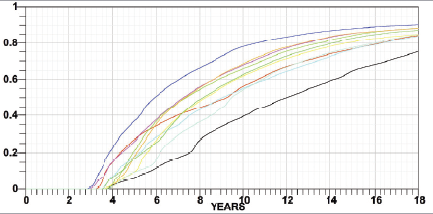
The sensitivity analysis can be understood with the help of the following graphs.
The right way of planning optimum production is to optimize creation of a gas field such that any more increase in production rate by raising the amount of wells will no longer add to an increase in current value revenue.
- Inflow Performance
- Tubing Performance
- Number of Wells
- Basic Production Pattern
- Economic Analysis
- Optimization
This topic also covers the gas field development in which the main features include the well performance, reservoir deliverability, gas field performance, present value calculations and optimum rate calculations. Let’s just understand them one by one.
Well Performance

Reservoir Deliverability
Tubing Pressure
Gas Field Performance
In order to avoid future mistakes and poor results, one must be sure that the planning and design is accurate. It is the task of the reservoir engineer to make sure that the design is accurate and how many wells and other items should be used.
Parameters and Their Purposes
The parameters that have to be optimized are α, β and. The points in time are mathematically represented this way by alpha, beta and gamma.
The parameter alpha is used for the value between zero and 1.2, the beta is used for the value between zero and 0.75 and the parameter gamma is used for the value between 0 and 1. The parameter gamma is the measure of the total amount of gas that is still being produced until the end of the field’s economic life at any point in the time during the reducing period. With these special units, the future life of the gas field can easily be represented mathematically. If we want to express the future economic value of gas production, these mathematical units may be used to get the present value of the future gas field.
Overview of Gas Field Performance Prediction
Estimation of Gas Reserves
There are two common methods that are used for the gas reserves estimation. You can never be sure about the estimation of the gas reserves. The extent of this uncertainty depends on a few things that are mentioned below:
- Reservoir type
- Source of reservoir energy
- Assumptions made during the process
- The required technology
- Experience and understanding
Common Methods
- First of all the volumetric estimation after the discovery is the solution to the estimation.
- Secondly, when depletion continues the material balance may give a second method. This is the optimum method (PSC 2008).
A few factors that affect the efficiency of these two methods are:
- Temperate to strong water drive
- Low standard permeability
- Multifaceted inner architecture and deprived lateral or vertical continuity.
Methods of Estimation of Gas Reserves
Volumetric method
The volumetric method is the most common method which is used after the detection premature stages of production. Then in this method the standard reserve equation with suitable selection of parameter include the area, thickness, water saturation, volume factor and then the recovery factor (Teufel 2004)..
Volumetric Estimate of Hydrocarbon
Let’s just study this method step by step.
- Step 1: Determination of the volume of rock from area and thickness.
- Step 2: Determination of average porosity.
- Step 3: Determination of water saturation.
- Step 4: Volume correction at the room temperature.
Uses of Volumetric Estimation Method
- It is useful for the estimation of gas reserves at any time of depletion.
- It is useful in the development period.
- It provides significant checks on gas estimates obtained from the material balance method.
Material Balance Method
The material balance method can be functional after getting the certain amount of production data. For example:
- Production amount
- Reservoir force and temperature
- liquefied analysis data
- Log data and Core data
- Drive Mechanism
Pressure Decline Curve Method
The pressure decline curve method can provide three very important things:
- Remaining gas and oil reserves
- Future expected production rate
- Lasting production life of well or reservoir
The wells can not be modified and the drainage that takes place is steady throughout (Robinson 2002).
Determination of Area
The limit that frequently has the maximum inconsistency in the reserve estimation is the area selected to signify the area extent of the reservoir.
- In Petrobangla, area for gas reserve inference is measured at 3.14 Sq. Km or 716 acre. This comes to the area inside a circle of 1km radius.
- This area was initiated by the experts from past Soviet Union.
- Oil & Gas Development Corporation, state possesses E & P organization of Pakistan was recognized at some stage in early sixties with scientific support from previous Soviet Union.
Formula to Get the Estimate of Oil Reserves:
- OIIP = Oil initially in Place
- OIIP = VR x Ф x 1/Bo x (1-Sw)
- VR = Rock Volume (Area x Average Thickness)
- Ф = Porosity
- Bo = Formation Volume Factor
- Sw = Water saturation
Now let’s say if the gas in reservoir occurred as the non associated gas, associated gas and solution gas then:
Case 1: Non Associated Gas
- G = VR x Ф x (1-Sw) x 1/Zi
- G = Gas in Place, VR = Rock Volume, Ф = Porosity,
- Tsc = Standard base Temperature in Kelvin (273 + C)
- Psc = Standard base pressure in Kpa,
- Ti = Initial Formation Temperature ( K),
- Pi = Initial Formation Pressure (Kpa),
- Zi = Gas Compressibility factor at Pi and Ti.
Case 2: Associated Gas
The gas that is associated with oil as the gas cap is actually known as associated gas. During the oil is being produced this gas remains in. This gas does not come out till the oil production is finished. The method of estimation is just the same as it has been described above.
Case 3: Solution Gas
This is the type of gas that escapes while the oil is being produced. To get a rough estimation of the volume of this gas the following formula is used:
- Gs = N x R
To find out Zi the following data is required
- Gas Composition
- Critical Pressure and Critical Temperature of single constituent of the gas from tank.
- Early Reservoir Pressure
- Original Reservoir Temperature
Inflow and Outflow Performance Relationship
The growth and reduction of a natural gas reservoir is reliant not merely on the geologic or engineering features of the tank, but is in addition reliant on the marketing stage of the gas. In other words, gas making cannot inaugurate until a gas sales deal has been signed. This deduces that a market is in attendance to acknowledge the gas at a particular cost. Also, in contract discussions, the most advantageous growth plan should be recognized as priori. For that reason, within the growth plan it will be compulsory to give an approximation of overall natural gas reserves, the well or wells output and efficiency, and the forecast of production rates to a spot of sales or move at a particular pipeline pressure.
When a field is initially exposed the gas-in-place can be predictable by relating volumetric. This technique necessitates some awareness of the area coverage and the petrophysical and gas properties of the tank. The substitute technique, material balance, necessitates at least a little pressure making narration to be capable to put together an approximation of gas-in-place. On the other hand, to conclude gas reserves necessitates some estimate of revival feature.
The revival factor is a strong purpose of the drive device. For reduction drive, the revival feature is on the order of 80 to 90% of the gas in place; despite the fact that for water drive systems the revival can be considerably less, something like 60% of the gas-in-place for a strong water drive. At a smallest amount, in reduction drive tanks, two pressure points are requisite to guess reserves. The first pressure taken at time of detection and the desertion pressure at which point the well or wells are no longer profitable.
The flow from the formation to the bottom of the well is governed by what we call inflow performance relationship and the flow from the bottom hole to the surface is signified by the outflow performance relationship. Before we do get in details we must know and understand the actually difference between the inflow and outflow performance relationship.
Inflow Performance Relationship
Inflow relationship is the relation between the rate of flow and the flowing bottom-hole pressure. The relationship is linear for tank producing at pressures above the bubble point pressure which actually is when the flowing bottom-hole pressure is superior than or equivalent to the bubble point pressure. Otherwise, this relationship can become a curve. When the inflow performance association is linear it can be signified with the productivity index. There are many method to determine the inflow performance relationship and for determining the future ones.
Outflow Performance Relationship
The outflow performance relationship includes the flow of liquid through the production tubular, the wellhead and the surface flow line. Actually the analyzing of fluid flow includes he determination of he pressure drop across every segment of the flow system. This is a very complicated kind of problem that is faced. There is no such solution to this problem to get it solved.
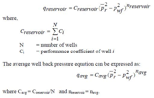
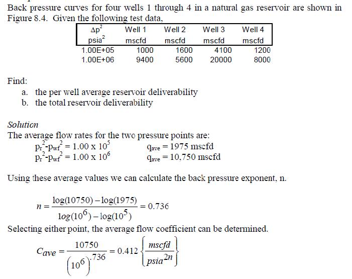
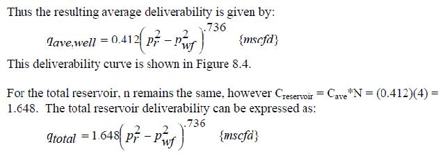
Back Pressure Equation
The deliverability of a well or tank cooperates a major role in the field growth. The determination of deliverability is connected to the totality of pressure drop that takes place from the pool to the position of sales. In estimating reservoir deliverability one should account for the disparity of proponent n and flow coefficient C in the back pressure equation. Characteristically, n is understood invariable for a well in the fullness of time.
On the other hand, as flow rate reduces the probability of turbulent flow will also reduce and the exponent will drift in the direction of one. In addition, the degree of commotion or skin can be at variance from well to well and as a consequence n will differ from corner to corner of a reservoir. The flow coefficient, C is affected by well spacing and well finishing point and therefore will also diverge with reduction. To settle on the whole reservoir deliverability the back pressure equation can be written as:
Here is an example as well that can make it easier to understand.
Example
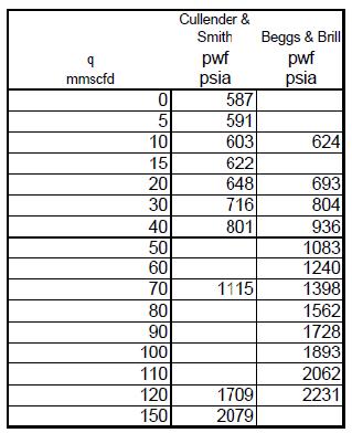
The Cullender and Smith Correlation
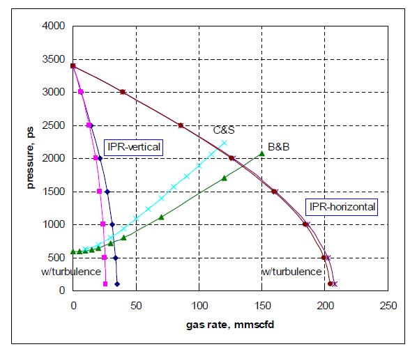
For equally the perpendicular and parallel well cases the wellhead pressure is invariable at 500 psia and the wellhead temperature at 75°F. The tubing dimension is 5.5” ID. The figure given below demonstrates the results for two connections for relationship; Cullender & Smith and the Beggs & Brill correlations, in that order. The Cullender & Smith correlation consequences are higher pressure losses and as a consequence are a lot conventional approach.
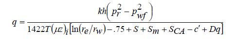
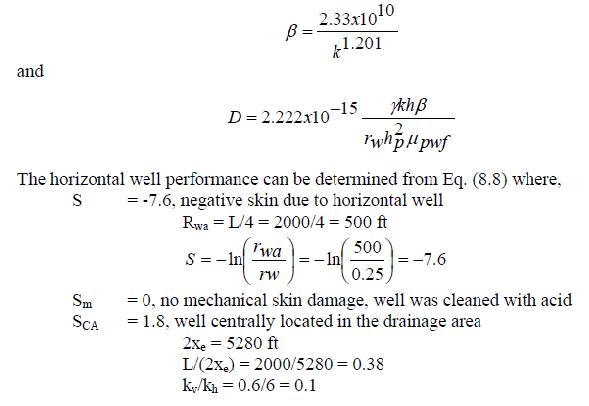
In vertical well inflow performance relationship equation above where,
S = 0, fully penetrating vertical well
Sm = 0, no mechanical skin damage, well was cleaned with acid
SCA = 0, well centrally located in the drainage area
c’ = 0, shape factor conversion constant for vertical well.
And for the non-Darcy flow component,
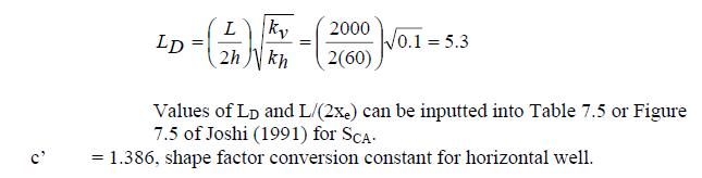
The figure given below illustrates the products for both the straight up and parallel well cases and with and without commotion. The figure shows the collision of instability in a horizontal well is negligible. The winding up is that horizontal well’s make available a way to lower well bore commotion, for the most part in high permeability gas tanks (Teufel 47). Also note the important dissimilarity in well presentation involving the vertical and horizontal well cases, something like a 3.5:1 ratio, a believable argument for horizontal wells.
Reservoir Deliverability
The “Deliverability” of a reservoir can be defined as the tank’s competence to generate in opposition to the constraints of the well bore and the method into which the well must flow. These restraints are blockades which should be prevail over by the force in the reservoir. Plummeting the magnitude of the well bore or raising the pressure of the system into which the well must generate, enlarges the confrontation to flow and for that reason decreases the “Deliverability” of the reservoir. The Deliverability Test allows estimates of flow rates for several line and tank pressures.
Deliverability test goes under more than a few names for instance “Back-Pressure Testing”, “4-Point Testing”, “Open Flow Potential Testing”, and “AOF Testing”. The terms “Open Flow Potential” and “Absolute Open Flow” refer to the hypothetical highest flow rate from the reservoir if the rub down face pressure were concentrated to atmospheric. A “Deliverability Test” more often than not necessitates the well to be generated at a number of rates. The flowing pressure at the sand face for every rate and the sand face pressure after increasing are then found. The pressure flow information is utilized to find out AOF or Deliverability (Shahab 33). Deliverability tests are exercised by authoritarian agencies to assign manufacture allocations and by tube operators to contract for gas procure.
Improving Deliverability
Deliverability can be enhanced by make use of fracturing, element actions, and huff ’n’ puff gas inoculation. Despite the fact that there is irregular information on the use of a variety of methods in gas condensate reservoirs with restricted and temporary achievement, it is easier said than done to discover details. Fracturing possibly will not give up predictable consequences if the plan does not include that the fracture may perhaps weight up with fluid condensate and that the condensate bank in the tank will restructure in the order of the fracture. Most chemical inoculation and huff ’n’ puff schemes will contain only short-range consequences for the reason that the bank will form. Reproductions show that a well-designed huff ’n’ puff CO2 shot (behind the field life with huge strikes) can supply an adequate amount of incremental PI to be profitable in a number of cases.
Gas Reservoir Performance
The given figure below demonstrates the features that affect the gas recovery.
If the reservoir is a congested component, we can also say that if it is not underlain by water then we can call it depletion reservoir. When the gas starts to generate the pressure comes down as we can clearly see in the figure given above. In case of ideal gas a straight line is formed. Production of gas is achievable from such a field up to a specific desertion pressure. This pressure is the lowest one in which a gas can still be produced.
When the line of abandonment pressure crosses he depletion line it means that 80 to 80 percent of gas is in the place or is being recovered. When the gas fields are underlain by water and when the pressure starts to come down the waters enters the reservoir and this helps to maintain the reservoir pressure. We can call it production or generation by water drive. We must know that there is a huge difference between oil and gas production and reservoirs.
In the case of gas reservoir, water drives fields do not have high revival features than reduction type fields. Most of the gas is usually left behind in the pores of the rock. We call it residual gas as it is left behind at the end. When the water drive decreases in potency the recovery of gas is much more efficient. It is basically the responsibility of the reservoir engineer to make the estimate and help in future plans of gas recovery.
Tubing Performance
Tubing performance is basically the vertical flow performance of gas in the reservoir. We must know that well flowing pressure is different from the tubing head pressure. Here is a figure that will help us to understand the tubing performance more easily.
The decrease in well flow rate is actually caused by the tubing performance. For higher production rates, we have got to know that further than a particular production rate dependant on the tubing extent, an enhancement in “square drawdown” can never perk up the production rate. The tubing acts practically as a strangle nipple as the rates attain the upper limit of flow conditions. It is obvious that the maximum production rate from 5 inch tubing is higher than that of 3 inch tubing. The given inflow graph also helps us to determine the tubing performance.
Tubing Performance
When we talk about the inflow and tubing performance combined then the intersection of the inflow performance curve and tubing performance curve gives or finds out the production rate at the conditions like:
- Static Reservoir Pressure
- Type of well inflow performance
- Tubing size
- Tubing head pressure needed
It is clear that the highest production rate that we get from a 3 hours production test or experiment is just about the same as we can expect from alleviated conditions. We can say that this sure is a coincidence. The failure acquired by the stabilized inflow performance will then be remunerated by the augment because of larger tubing size. It is achievable to make the estimate of the number of tubing performance curves. It is the reservoir engineer who is responsible for all the tasks and advantages and disadvantages received from the test of gas recovery. This is not only a technical aspect but is also economical.
Reservoir Performance Prediction
Reservoir performance analysis and prediction is incorporated in the project setting up, plan management and multi punitive incorporated cooperation approach. This means that we review the customer’s requirements, then invent and carry out a fit for reason work opportunity to help the consumer put together good decisions for reservoir development or reservoir management.
Depending on the character of the difficulty, the plan aims and the quantity of time and information obtainable we can use standard reservoir engineering such as material balance or decline curve analysis in addition to up to date tank simulation modeling. We may also make use of an amalgamation of methods to give better assurance in the consequences, for instance material balance supported by analogue field performance statistics or tank simulation held up by decline curve analysis.
Perfect performance prediction of miscible improved oil recovery (EOR) plans or CO2 confiscation in used up oil and gas tanks relies in part on the capability of an equation-of-state (EOS) model to effectively correspond to the assets of an extensive range of mixtures of the occupant fluid and the inserted fluids or fluids. The combinations that form when gas relocates oil in an absorbent medium will, in a lot of cases, vary considerably from works generated in swelling tests and additional normal pressure/volume/temperature (PVT) experimentations.
Multicontact tests (e.g., slim tube displacements) are frequently exercised to state an EOS model ahead of application in performance assessment of miscible disarticulations. On the other hand, no understandable knowledge is present of the impact on the consequential accurateness of the chosen classification process when the liquid explanation is consequently included in reservoir simulation.
Analytical and arithmetical techniques for predicting the performance of a gas-injection procedure depend on an EOS to forecast the stage performance of the combinations that shape in the way of a disarticulation process. The function of the phase performance in relation to mathematical dispersal in compositional reservoir reproduction has been pointed out up to that time by Stalkup. In recent times a technique to enumerate the interaction of the phase performance and arithmetical diffusion in a finite-difference reproduction of a gas-injection process. By analyzing the stage behavior of the injection-gas/reservoir-liquid scheme, a calculation of the impact, referred to as the dispersive detachment, can be computed. The dispersive distance is helpful when scheming and deducing large-scale compositional tank simulations.
Sensitivity Analysis
To carry out sensitivity analysis, a tank engineer has to reduce the amount of uncertainty issues and factor levels, which possibly will over and over again show the way to inaccurate conclusions. To optimize gas reservoir performance, a representation of the tank is essential. We have a preference to employ the simplest model that is capable to forecast storage-reservoir presentation as a purpose of the amount and locations of wells, density horsepower, and cushion gas volume.
Even though models combining material balance with systematic or experiential deliverability equations may be utilized in a few circumstances, a reservoir-simulation representation is more often than not most excellent, owing to its suppleness and its capability to handle well intrusion and multifaceted reservoirs accurately. Different but most favorable growth patterns are obtained for different fields and that for any specified field a cautious analysis of the different physical parameters will be required before such an optimum pattern can be put together.
It is significant to standardize the model beside chronological making and pressure data; we have to demonstrate that the model repeats past reservoir performance perfectly before we can utilize it to predict future performance with dependability. On the other hand, even adjusting the model by the past matching past performance may not be sufficient. It is the knowledge that information attained for the duration of primary reduction of a reservoir is often not enough to forecast its performance under storage operations.
Most important production over a lot of years may mask covered or dual-porosity behavior that significantly affects the ability of the reservoir to deliver large volumes of gas within a 3 to 5 month period. Wells and Evans presented a case narration of the Loop gas storage field, which showed this performance (Katz and Elenbaas 44). It may be essential to put into practice a program of coring, logging, pressure-transient testing, and/or simulated storage production/injection testing to differentiate the reservoir precisely.
It is the responsibility of the reservoir engineer to be careful and cautious while performing any of the test and predicting any further performances.
Predicting Reservoir Performance
Problem
Reservoir/well information.
Contract considerations dictate gas delivery at a maximum rate of 3.12 mmscfd per well against a wellhead pressure of 500 psia. The plan is to produce two wells at this maximum rate until such a time when the reservoir pressure has declined to the point where this rate can no longer be sustained. Thereafter, the production rate will decline with time.
The objective is to predict the reservoir performance of the field beginning at t = 2 years and lasting until abandonment, estimated to be qa ~ 300 mscfd.
Nomenclature.
Solution
Constant rate Period
Step 1: Use Cullender & Smith correlation (and Tr, Twh, Tubing ID, depth, gas gravity) to determine the minimum bottom hole pressure, Pwf that will sustain a flow rate of 3.12 mmscfd per well against a wellhead pressure, Pwh of 500 psia. This was done in a MATLAB program to automate the process.
Pwf to sustain given rate = 618 psia.
Step 2: Compute corresponding reservoir pressure pr from pseudo-steady state equation for radial flow of real gases at low pressures. Since viscosity and z-factor are pressure dependent, this process is done by an iterative procedure. Process is initiated by assuming a reservoir pressure between Pr and Pwf.
Assume initial value for Pr.
Assumed Pr = 1000 psia
Compute an average pressure of Pr and Pwf using the root mean squared method.
Pave = 831 psia
Determine corresponding μ and z values based on this average pressure.
zave = 0.931, μave = 0.0139cp,
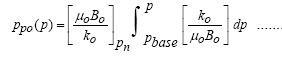
Calculate new pr value using pseudo-steady state equation.
Pr2 = pwf2 + 1422
![]()
[ln(re/rw)- 0.75 + s’] pr = 895 psia
Compute difference between initial and calculated pr values.
Difference = 1000 – 895 = 105 psia
Repeat steps 2.2 through 2.5 using calculated prn as initial prn+1 until difference = 0.
Final pr value = 895 psia
Step 3: Calculate corresponding value of cumulative gas using material balance equation for Gp.
Gp =G[Pi/Zi-P/Z/PI/ZI]
Gp = 7.73 Bscf
Step 4: Calculate actual gas produced during the time period.
Actual Gp produced during constant rate time period = 7.73 – 3.92 = 3.81 Bscf
Step 5: Calculate estimated time period to produce these reserves, t =Gp/q*N
t = 610 days or 1.67 yrs
Declining rate Period
Initiate Procedure by applying values from previous constant rate analysis.
pr = 895 psia Gp (cumulative) = 7.73 Bscf qtotal = 3.12 * 2 = 6 mmscfd
Step 6: Decrease pressure by an assumed value. Here, 100 psia is used.
New pr = 795 psia
Step 7: Determine z factor for new reservoir pressure and calculate p/z at this pressure.
z = 0.935; p/z = 795/0.935 = 850 psia
Step 8: Update the cumulative gas produced for the new reservoir pressure.
Gp = 8.48 Bscf
Step 9: Calculate incremental cumulative production for the time period, ΔGp.
ΔGp = 8.48 – 7.73 = 0.75 Bscf
Step 10: Identify the intersection point between the inflow and outflow performance i.e. gas rate where both the inflow and outflow produce the same bottom hole well flowing pressure. This is single gas rate at the specified wellhead pressure.
Gas rate = 2.13 mmscfd
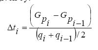
Step 11: Calculate log average reservoir flow rate over the time period, log qave = (log qn-1 + log qn) /2.
log qave = 3.65 mmscfd
Step 12: Calculate time period, t =ΔGp/qave
t = 205.4 days (0.56 years)
Step 13: Repeat steps 8 through 14 with new values for reservoir pressure, gas rate and cumulative production until economic limit is reached.
Step 14: Performance prediction – create table and rate vs. time plot to show performance over reservoir over time
Performance Predictions
Assumptions
- Both wells have identical producing characteristics.
- Static bottom-hole pressure, pr is equal to the average reservoir pressure.
- Static bottom hole temperature is equal to bottom hole well flowing temperature.
- Constant skin factor at during production.
Optimization of Natural Gas Field Production
Gas and oil productions are not same, there is usually a misconception occur that oil and gas reserves are same but there is a need to identify the difference in oil and gas reserves. Oil and gas reserves and production is different not just because of different physical characteristics and properties but they are also different purely for economic reasons. Optimum level oil field production is possible by applying different techniques but optimum gas production is directly linked with market via pipeline.
Therefore the reservoir behavior doesn’t always help in determine best depletion pattern as there is a strong restriction that market must accept provided level of gas. In gas field, there is a strong bond and relationship exists between the production and marketing phases of the gas. In gas field, some restrictions are always involved and production could not be started until the gas sales contract has been signed. There are few basic parameters which are required to be determined before the development has begun.
Determining these parameters is not possible in case of oil production as oil doesn’t pose a direct link with the market. The detailed knowledge of these parameters in oil field and in the planning of gas field development pattern in linked with gas sales signed document is at risk to many uncertainties. In later sections of this paper various steps have been simplified in order to avoid undue complications in gas development field. As, it is stated above, that there is a big vast difference between gas and oil reservoirs due to economic reasons. In case of oil reservoirs water drive usually have a high recovery factors than depletion type fields. In case of gas reservoir this process becomes reverse.
The reason of this effect is water doesn’t displace all the gas in gas reservoir. An appreciable amount of gas is usually trapped by capillary forces in the spaces of the rock and is by-passed. This gas is usually termed as residual gas and expressed in percentage as 40 percent to 20 percent. IF the water drive decreases in the strength in result of which ultimate recovery will be higher and the same case will occur with a weak water drive, ultimate recovery in weak water drive may be little higher in case of depletion pattern. Water drive strength is highly depend son three factors which are listed below:
- Permeability of formation
- Strength of water drive
- Time Factor
Offtake Pattern
The offtake pattern of a gas field is restricted by 2 constraints Firstly, the off take should be such that the market can soak up the gas that is generated and this can lead to a constraint of the rate at which making can built be produced. Secondly, the rate of build up may be constrained by the corporeal capabilities of boring wells and building amenities to carry the gas from well head to pipeline. The utmost off take rate of the field may also be restricted by gas field economic deliberations. The following figure helps us to understand it easily.
The economic results can never be the same if the interest on principal is taken in account.
Basic Production Pattern
In this pattern the economic result of future gas production is predictable on the source of the field of production in which no additional drilling takes place. The more the wells are drilled the production rate will increase. The total rate of making is actually calculated by multiplying the number of wells and highest production rate per well. For example if in a gas field the number of wells that have been drilled then the future production will consist of a period of steady rate all through which well potential go beyond the highest allowable rate. In the figure given below a particular system of units has been used to correspond to the values of production rate on the perpendicular axis and increasing gas production on the parallel axis.
On the horizontal axis cumulative gas recoveries have been planed and are articulated in a unit of gas production which stands for the total quantity of gas that is found from the start of decline period until the profitable limit of field is reached which actually is the maximum amount of gas composed during the decline period. With the help of this particular system of units, which are in actual fact dimensionless, the prospect life of any particular gas field may be represented scientifically. In order to state the future economic value of gas creation; this system of unit may be used as explained in the present value calculation section.
Present Value Calculation
The financial value of the future gas can be expressed in terms of funds by calculating it’s self styled “present value”. We can compute the present value of the potential amount to be expected by multiplying it by the “deferment factor”.

In the example given above we can see how the present value can be calculated. The total annual production rate is multiplied by a financial value and the sum of 3 postponement factors D1, D2 AND D3 valid for the total production obtained at some stage in the steady rate period, the compressor time, and the decline period correspondingly. The last value calculated is the cash generation per unit of gas that is sold.
Optimum Offtake Patterns
In order to understand this we must first know what optimization is. Optimization is the optimum production rate of a gas field reached by the increase in the production rate by increasing the mount of wells that no longer supply to an increase in present value profit. This is mathematically expressed by putting the degree of difference coefficient of the present value profit P* with regard to the number of wells that are equal to zero. It is clear that the production rate depends on the values of parameters alpha, beta and gamma and the value of the parameter is the most important of all. It is achieved in the end by dividing the annual cash generation per well as shown in the equation given above of optimum rate. The value of the other parameter expresses the ratio between the compressor speculation and the well savings.
Example
The highest graph shows the optimum growth pattern for a field having a large part of reserves which can be formed before the setting up of compressor is necessary. The perfect example of optimum off take pattern is given below in the form of diagram.

After the experiments and calculations a very complex field development pattern is seen with a reduced conductivity field where only very limited production will happen previous to the period throughout which compressors must be installed in order to distribute gas to the pipeline.
From the example that has been discussed it gets very clear and understandable that depending on the financial circumstances, different but most favorable growth patterns are obtained for different fields and that for any specified field a cautious analysis of the different physical parameters will be required before such an optimum pattern can be put together. The reservoir engineer’s task is to tell the range of patterns that are in his knowledge right after the discovery of the field that will help the marketers to make the gas sale contracts in the right manner which is the task of the gas sale contactor.
Works cited
Ikoku, C, Natural Gas Reservoir Engineering, Krieger Publishing Co., Malabar, FL, 1992.
Poettman, F.H, Method for Predicting the Back-pressure Behavior of Low Permeability Natural Gas Wells,” Trans.AIME 210, 1957: pp 302.
J. Van Dam, “Planning of Optimum Production From a Natural Gas Field,” 1967.
Chi U. Ikoku, “Natural Gas Production Engineering”, 1984.
Shahab Mohaghegh, Virtual Intelligence and Its Applications in Petroleum Engineering, JPt, 2000, pp: 33-45.
Nabil Al-Bulushi,Predicting water saturation using artificial neural networks (ANNS), Innsbruck, Austria, 2007, P: 57 – 62.
Camacho-Velázquez, Inflow Performance Relationship (IPR) For Solution Gas-Drive Reservoirs—Analytical Considerations,SPE, Texas A&M U, 2007, P:58.
Katz, Elenbaas, “Design of Gas Storage Fields,” Trans. AIME 216, 1959, pp 44-48.
Teufel, L: “Optimization of Infill Drilling in Natural-Fractured Low-Permeability Gas Sandstone Reservoirs”, GasTips, 2004 p: 47.
Harstad, H.: “Drainage Patterns in Fractured Tight Gas Reservoirs,” Ph.D. Dissertation, New Mexico Institute of Mining and Technology, Socorro, NM, 1998, p 34.
Teufel, L: “Optimization of Infill Drilling in Natural-Fractured Low-Permeability Gas Sandstone Reservoirs”, GasTips, 2004.
Robinson, “An Effective Technique of Estimating Drainage Shape, Magnitude, and Orientation in a Low-Permeability Gas Sand,” SPE Paper 77742, presented at the SPE Annual Technical Conference and Exhibition, San Antonio, Texas, 29, 2002.
Short Course on Petroleum Reserve Estimation, Production, and Production Sharing Contract (PSC) DCE and PMRE, BUET, 2008 Gas Reserve Estimation.