Introduction
In economics, firms are known to produce their output to make profits. However, the costs of production normally affect this objective by reducing the profit margin a firm expects to enjoy. The relationship between production and costs is therefore an important relationship for firms because it virtually determines the volume of output it can produce before going out of business. Production essentially defines how much a firm is going to produce at a given cost. Most firms however prefer to produce at the optimum level to make more profits (in a perfect market) (Mankiw, 2008, p. 247). The determination of production levels in economics is normally undertaken using a production function which majorly includes aspects to do with costs, land, and labor (which in simple terms can be generalized as the factors of production) (Ricardo, 2005, p. 1).
From the above understanding (that costs affect the level of profits an organization can make), it is important to note that costs also determine the level of production a firm can undertake (Williamette, 2010). From this point of view, it is therefore correct to observe that costs and production are normally inversely related (Ricardo, 2005, p. 1). However, in analyzing costs, it is important to note that costs are subdivided into several categories. The main ones are fixed costs, variable costs, and total costs (Ryan, 2010, p. 1). Production and costs when analyzed from a general point of view refer to the same problem, but this ought to be understood through different avenues. In one avenue, production can determine the profit level a firm will enjoy by producing its output at a given level (but then, it has to determine the costs of producing at that level). In another avenue, a firm can determine its profit level, simply by controlling the costs it incurs in production (Ricardo, 2005, p. 1). These two avenues of analyzing a firm’s problem (when applied well) are bound to lead to the same conclusion (Ricardo, 2005, p. 1). The relationship between production and costs is however not as simple as it looks because it is affected by long-run and short-run production. From this understanding, this study seeks to establish the relationship between production and costs in the long run and short run. However, before we undertake this analysis, it is important to understand the conceptual analysis of long-run and short-run production and cost relationships in economics.
Conceptual Analysis
When comprehending the implications of long-run and short-run costs, it is important to note that in economics, such timeframes do not refer to the calendar time (Ricardo, 2005, p. 2). For instance, when analyzing a year as a distinct timeframe, it may seem quite long, when analyzed from a human perspective but when analyzed from a firm or economic perspective; a year can be a very short time. This analysis is true because it can be very difficult for a firm to change its stock capital into profits or products within a short time (Ricardo, 2005). In the same manner, it can be said that a month can be a very short time when analyzed from a human point of view, but when analyzed from a firm’s point of view, it can be very long, because it may be possibly easy for a firm to change labor and capital several times in a given month (Williamette, 2010). This would therefore mean that one month can be the long-run timeframe for a firm. Transitioning from the short-run to the long-run (or to the medium-run) all depends on how a firm manages the transition of the factors of production through these periods (Ricardo, 2005, p. 1). In other words, this refers to how a firm can change its costs from fixed costs to variable costs.
Long-run
In analyzing the relationship between production and costs in the long run; what companies try to do in the long run should be understood first. In comprehending this concept, we need to understand the different levels of production evidenced in the long run. In doing so; we need to understand production indifference curves and isoquant relationships. A production indifference curve is a representation of the substitution of inputs a firm can use in the production of a given output without changing the level of output (Ricardo, 2005, p. 1). This can be represented as follows:
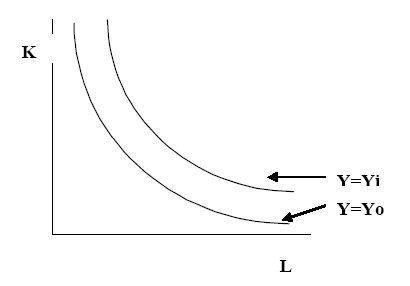
In the above diagram, we can witness two production indifference curves that are negatively correlated because they show the different levels of tradeoffs a firm can make for substituting capital for labor without changing the level of output. It is however important to note that the farther away the isoquants are from the origin, the higher the level of output (Ricardo, 2005, p. 1). It is also important to note that the slope of the indifference curve is normally known as the marginal rate of technical substitution (Ricardo, 2005, p. 1). With these consideration factors, we should understand that firms are normally limited by costs that are incurred when producing at a given level of output. This is true because firms are normally not endowed with the capability of spending whatever amount of money they want in production. This also means that firms should determine very carefully what they can spend at a given production level.
Normally, for firms to determine their expenditure, they simply have to engage a direct additional process of doing so, but this need not be the case for all firms (Williamette, 2010). Ricardo (2005, p. 14) explains that:
“What this means is that firms calculate their total expenditure by multiplying the price per unit of input with the number of inputs they use. For example, if a company uses labor and capital, its expenditures are going to be the wage multiplied by the number of workers and the interest rate or the number of capital multiplied by the price of capital used”.
Therefore, in determining expenditures, the following formula can be employed: E= (W*L) + (R*K) (Ricardo, 2005, p. 14). E would be the costs; W is the wage rate; L is the number of personnel used; R is the interest rate and K is the total number of units of capital used in the entire production process (Ricardo, 2005, p. 14). This equation implies that a firm can use several expenditures in any given production level. For example, a firm can decide to use a higher expenditure level because it uses more input and produces a higher output level.
From the above analysis of production, when understood through the analysis of Ricardo (2005), we can see that “in the long-run, firms tend to maximize on the marginal rate of technical substitution or the slope of the isoquant to the ratio of the relative input prices, the slope of the expenditures line” (p. 15). In other words, in the long run, a firm would be trying to establish the following balance MRTS = W divide by R (Ricardo, 2005, p. 14). In this equation, w remains to be the wage rate and r also remains to be the interest rate. In the long run, therefore, firms would often try to maintain this balanced equation; failure to which, the firm would not be minimizing the costs incurred in producing the output. Consequently, the firm would be inefficient (Ricardo, 2005, p. 14). This situation can be depicted by the following diagram:
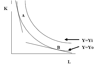
The diagram represents several production levels, but not all of them are efficient. For instance, point A can be termed as inefficient because the marginal rate of technical substitution is not equal to the prices of the inputs (or the costs of production). In the same manner, point B can also be said to be inefficient because the marginal rate of technical substitution is similarly not equal to the costs of inputs (in any case, the Marginal rate of technical substitution is less than the total costs of input). However, point C does not suffer the same fate because the marginal rate of technical substitution is the same as the total costs of inputs. This point best explains the relationship between production and costs in the long run.
Short-run
The simplest type of short-run production and cost relationship can be explained through the inclusion of one fixed and one variable cost. The following equation best represents this situation, Q=f (L, K) (Williamette, 2010). In this equation, the firm has determined a given level of production level which can only be increased if the labor employed is increased as well (because the level of a fixed input is unchanged) (Maurice & Thomas, 2008, p. 296). It should also be noted that increasing the capital input in the short-run causes other input factors to be more productive than if the initial value of the capital was maintained (Maurice & Thomas, 2008, p. 296). For instance, an increase in the capital input from 2 to 3 units is likely to result in a higher level of output, if the labor usage is increased (because the production curve is likely to shift upwards if capital is increased) (Maurice & Thomas, 2008, p. 296). For example, with three units of capital, a higher output or production level can be realized, as opposed to a situation where only 2 units of capital are used.
In concentrating on labor as a variable cost, Maurice & Thomas (2008) explain that “While increasing the quantity of capital boosts labor productivity and output at every level of labor usage, the productivity gained will be even greater if the additional capital input embodies advanced, state-of-the-art technology” (p. 300). In other words, a higher technological input simply increases the level of variable input because most of the time, old capital is based on older and less efficient technology (Ryan, 2010). There have been real-life examples where increasing capital productivity through technological means has consequently led to an increase in productivity. For instance, the petroleum industry in the Western world is currently experiencing high levels of productivity through the diversification of its oil exploration activities and the upgrading of its exploration facilities (Maurice & Thomas, 2008, p. 300). Consequently, it can be evidenced that the production capacity of such firms has increased over the months while variable costs such as labor, and energy have either remained constant or decreased to a significant level (Maurice & Thomas, 2008, p. 300). Such high production levels have been attributed to the high investments in technology during the production process in the 90s (Maurice & Thomas, 2008, p. 300). This kind of relationship explains the unique relationships firms face about production and costs in the short run.
Conclusion
In the short run, managers are normally equipped with just a few fixed and variable inputs. The production levels in the short run can be changed by hiring a few more employees or shifting the level of raw materials used in the production process. However, plant and equipment (fixed costs) used do not normally vary in the short run. It should also be known that in the long run, the decisions in production are still the same as the short-run, only that all the input costs can be varied in the long run. Moreover, it should also be understood that when a firm changes its production capacity or adds new plant and equipment (in the long run); the production decisions faced become similar to the short-run. From this analysis, it is important to note that the costs structure in production changes, depending on the timeframe in consideration.
References
Mankiw, G. N. (2008). Essentials of Economics. London: Cengage Learning.
Maurice, S., & Thomas, C. (2008). Managerial Economics w/ CD (9th ed.) New York, NY: McGraw-Hill.
Ricardo, H. (2005). Production, Costs, and their Relationship. Web.
Ryan, M. (2010). Production and Cost Principles of Microeconomics. Web.
Williamette. (2010). Cost and Production.