Review Correlation and Regression in Education

Assignment

Exploratory Data Analysis of Chamorro-Premuzic.sav

Age. Descriptive statistics (Table 1) shows the age of respondents varies from zero to 43 years with a mean of 19.60, mode of 18, and a standard deviation of 3.448. In distribution, the age of respondents has positive skew (skewness = 2.35) and a sharp peak (kurtosis = 17.989).

Table 1.

Gender. The frequency distribution of gender (Table 2) indicates that out of 424 respondents, females comprised 71.4% (307), while males constituted (27.2% (117). However, the data have six missing values forming 1.4% of valid respondents.

Table 2.

Students’ Personality Traits

Table 3 depicts descriptive statistics of personality traits of students, namely, neuroticism, extroversion, openness, agreeableness, and conscientiousness. The trait of neuroticism has a mean of 23.63, mode of 24.00, and median of 24.00 with a standard deviation of 8.60. With maximum and minimum values of 0 and 44, respectively, the distribution has no skewness (0.005), but it has negative kurtosis of -0.312. The trait of extroversion has a mean of 30.10, median of 31.00, and mode of 33 with a standard deviation of 6.32. Extroversion score ranges from 5 to 46 with negative skewness (-0.459) and a positive kurtosis (0.671). The trait of openness has a mean of 28.83 (SD = 6.22), a median of 29.00, and a mode of 29 with maximum and minimum values of 14 and 46, correspondingly. The distribution of openness has a positive skew of 0.161 and a negative kurtosis of -0.462. The trait of agreeableness among students has a mean of 46.52 (SD = 7.45), a median of 47.00, and a mode of 50. The distribution has a negative skew of -0.136 and a positive kurtosis of 0.204. The trait of conscientiousness has a mean of 30.20, median of 30.00, and mode of 34.00. The distribution has a slightly positive skewness (0.029) and a positive kurtosis of 0.239.

Table 3.

Expected Lecturers’ Personality Traits

Descriptive statistics (Table 4) show that students have different expectations regarding the personality traits of their lecturers. The train of neuroticism ranges from -30 to 25 with a mean of -21.68, median of -24, and mode of -30 with a positive skew of 1.91 and a positive kurtosis of 4.95. Concerning the trait of extroversion ranges from -6 to 28 with a mean of 12.96, median of 13.00, and mode of 10 without skewness but a negative kurtosis of -0.213. Openness is the trait that ranges from -15 to 30 with a mean of 8.77, median of 8, and mode of 6. The trait of agreeableness ranges from -21 to 29 with a mean of 8.89 (SD = 9.58) with a negative skewness of -0.154 and negative kurtosis of -0.467. Conscientious has values that range from -8 to 30 with a mean of 6.29 (SD = 7.72) with a negative skewness of -0.496 and a negative kurtosis of -0.115.

Table 4.

Scatter Plots

Students’ Agreeableness/Lecturers’ Agreeableness

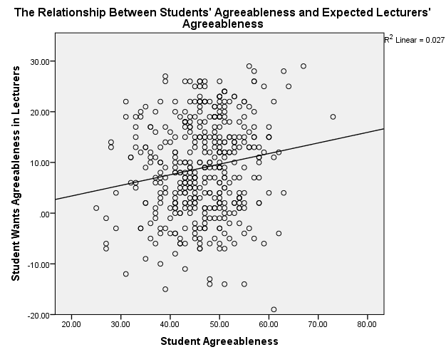
Figure 1. Scatterplot of Students’ Agreeableness and Expected Lecturers’ Agreeableness

Students’ Extroversion/Lecturers’ Extroversion

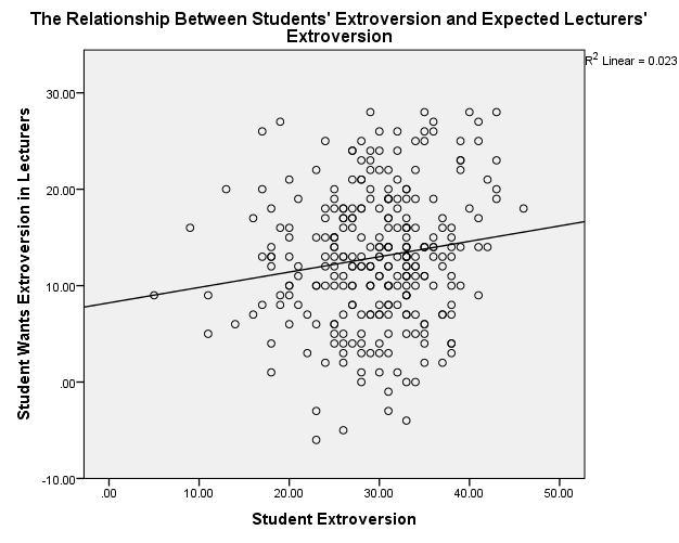
Figure 2. Scatterplot of Students’ Extroversion and Expected Lecturers’ Extroversion

Students’ Agreeableness/Lecturers’ Extroversion

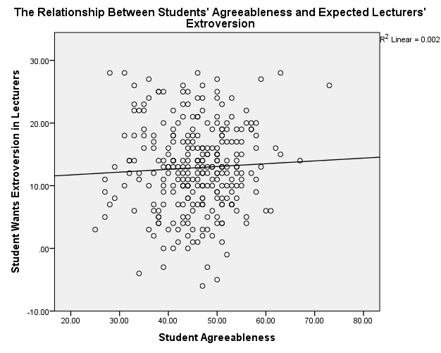
Figure 3. Scatterplot of Students’ Agreeableness and Expected Lecturers’ Extroversion

Students’ Extroversion/Lecturers’ Agreeableness

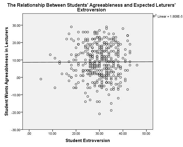
The scatterplots show that students’ agreeableness and extroversion have a positive relationship with varying strengths of relationships. In figure 1, students’ agreeableness accounts for 2.7% (R² = 0.027) of the variation in lecturers’ agreeableness, while in figure 2, students’ extroversion explains 2.3% of the variation in lecturers’ agreeableness. Students’ agreeableness has negligible effect because it accounts for 0.2% (R² = 0.002) of the variation in lecturers’ extroversion. Moreover, students’ extroversion does not affect because it explains 0% (R² = 0.000) of the variation in lecturers’ agreeableness.

Correlation Analysis

Since the missing values are present in data, the analysis handled them by pairwise deletion. George and Mallery (2016) explain that the pairwise deletion of missing values is advantageous because it does optimize not only data but also increases the power of analysis. In correlation analysis, the study employed a two-tailed test because the relationships between variables can be either negative or positive. Table 5 reveals that students’ extroversion has statistically significant but weak positive relationship with the expected lecturers’ extroversion (r = 0.153, p = 0.010). However, students’ extroversion has no statistically significant relationships with students’ agreeableness (r = 0.080, p = 0.106) and the lecturers’ expected agreeableness (r = 0.004, p = 0.932). Students’ agreeableness has no relationship with the expected lecturers’ extroversion (r = 0.05, p = 0.412) but with statistically significant positive relationship with the expected lecturers’ agreeableness (r = 0.164, p = 0.001). The expected lecturers’ agreeableness has statistically significant positive relationship with the expected lecturers’ extroversion (r = 0.118, p = 0.049).

Table 5.

Regression

The regression analysis to predict the effect of students’ extroversion of the expected lecturers’ extroversion meets the assumptions of linearity of relationship, lack of collinearity, and significant outliers are absent. The R-value is similar to that of the correlation because it indicates there is a weak relationship between students’ extroversion and the expected lecturers’ extroversion (R = 0.153). The regression model shows that students’ extroversion explains 2.3% of the variation in the expected lecturers’ extroversion (R² = 0.023) (Table 6). The regression model is statistically significant in predicting the influence of students’ extroversion on the expected lecturers’ extroversion, F(1,279) = 6.687, p = 0.010 (Table 7). Coefficient shows that an increase in students’ extroversion by a unit causes the expected lecturers’ extroversion to increase by 0.160 (Table 7), which is statistically significant at the alpha level of 0.1 (two-tailed test).

Table 6.

Table 7.

Table 8.

Multiple Regression

Multiple regression analysis of the effect of age, gender, and students’ extroversion on the expected lecturers’ extroversion met the assumption of linearity of relationship, a continuous scale of the dependent variable, lack of autocorrelation, and absences of significant outliers. Table 9 shows that there is a weak relationship between the independent variables and the dependent variable (R = 0.168). Moreover, regression analysis indicates that age, gender, and students’ extroversion accounts for 2.8% of the variation in the expected lecturers’ extroversion (R² = 0.028).

Table 9.

The regression model (Table 10) is statistically significant in predicting the effect of age, gender, and the expected lecturers’ extroversion, F(3,276) = 2.673, p = 0.048.

Table 10.

Table 11 reveals that only students’ extroversion is a statistically significant predictor of the expected lecturers’ extroversion (β = 0.161, p = 0.010). Age (β = 0.019, p = 0.866) and gender (β = 1.036, p = 0.265) are not statistically significant predictors based alpha level of 0.05.

Table 11.

Pearson Correlation

An area of research interest comprises factors that influence economic growth and development in various countries. The inflation rate and the gross domestic product are two variables that correlation analysis can determine the magnitude and direction of the relationship. The inflation rate exists on a ratio scale because its measurement is on percent changes, while the gross domestic product is on an interval scale since its values are in dollars. The mock finding is that the inflation rate has a moderately negative effect on the gross domestic product of a developing country (r = -0.4, p = 0.031). R² of 0.16 (r²) indicates that inflation explains 16% of the variation in the gross domestic product. The economic resilience of a country is a third variable that mediates the effect of inflation on the gross domestic product.

Spearman’s Correlation

Spearman’s correlation can assess the strength and course of the relationship between the degree of experience and the proportion of sales that employees make per year. The degree of experience exists on an ordinal scale that ranks years based on five-year categories. In addition, the proportion of sales is on an ordinal scale of 10% increments. The mock finding of Spearman’s correlation shows that there is a positive relationship between the degree of experience and the proportion of sales among employees in an organization (ρ = 0.65, p = 0.029). The effect size indicates that the relationship is strong because the degree of experience explains 42.3% of the variation in the proportion of sales. However, age is a third variable that confounds the effect of the degree of experience on the proportion of sales.

Partial Correlation vs. Semi-Partial Correlation

Population, inflation, and gross domestic product are three variables that I can use in calculating partial correlation. The similarity between the partial correlation and semi-partial correlation is the control effect of one or more third variables. However, the difference is that partial correlation control for the effect of a third variable on both correlating variables, while the semi-partial correlation control for the effect of a third variable on either of the correlating variables (Darlington & Hayes, 2016). In this case, partial correlation entails controlling for the effect of population on the relationship between inflation and the gross domestic product. Comparatively, semi-partial correlation involves controlling the effect of the population on either inflation or the gross domestic product in their relationship. In research, I would use partial correlation because it controls for the effects of population on both inflation and the gross domestic product.

Simple Regression

The unemployment rate and the crime rate are two variables that I could use in calculating a simple regression analysis. The unemployment rate is the proportion of people unemployed in the labor market, while the crime rate represents the fraction of reported crimes in the population. Both the unemployment rate and the crime rate exist on a ratio scale. The unemployment rate would be a predictor because it influences the crime rate, the outcome variable. In simple regression, R² would indicate the extent to which the unemployment rate explains the variation in the crime rate.

Multiple Regression

Property price, the interest rate, distance from the city, and the number of rooms are four variables that I could use in performing multiple regression analysis. Property of prices represents the value of houses in dollars on a ratio scale. The interest rate is the proportion of money charged on loaned money, which is on an interval scale. The distance from the city in kilometers exists on an interval scale. The number of rooms, which is on a ratio scale, shows the size of the property. Interest rates, distance from the city, and the number of rooms represent the predictor variables since they are independent variables that influence the property price, which is the outcome variable. The best method that I would use in multiple regression is stepwise because it allows the selection of significant predictors in a model. R² would depict the collective effect of all predictor variables on the property price, whereas adjusted R² shows the cumulative influence of weighty predictors on the outcome variable.

Logistic Regression

The price of a product, the availability of a product, and the choice of customers are three variables that could be analyzed with logistic regression. The price of a product exists on a continuous scale of dollars, while the availability of a product and the choice of customers are on a categorical scale (dichotomous scale of no or yes). The choice of customers is an outcome variable because it exhibits consumer behavior and is on a dichotomous scale. The price and the availability of products are predictor variables since they influence the consumer behavior of preferences. I would use the regression method of entering because it includes all predictors in the modeling of the regression equation. The regression output would generate Nagelkerke R Square, which indicates the degree to which the price and the availability of products influence consumer behavior. Moreover, the regression output would create coefficients for each predictor indicating magnitude, the direction of influence, odds ratio, and significance.

References

Darlington, R. B., & Hayes, A. F. (2016). Regression analysis and linear models: Concepts, applications, and implementation. New York, NY: The Guilford Press.

George, D., & Mallery, P. (2016). IBM SPSS statistics 23 step by step: A simple guide and reference (4th ed.). New York, NY: Routledge.