Economics is a subject that examines the behavior of different economic agents as they try to achieve their objectives in the face of resource constraints. Resources are scarce and therefore economic agents need to make choices. The process of making choices is important because it determines whether or not the economic agents achieve their objectives. Mathematics is an important tool in aiding economic agents to make their decisions. This paper examines four different types of functions: linear, inverse, curvilinear, and functions of two independent variables, and their applications to economics.
Inverse Functions
An inverse function is a function that is expressed as a reverse of the original function. For instance, if the original function gives y as the dependent variable and x as the independent variable, the inverse function will give x as the dependent variable and y as the independent variable. Thus, if the original function was: y = f(x), the inverse function is: x = f-1(y) The function y = f(x) implies that different values of x will give unique values of y whereas the inverse function x = f-1(y) implies that different values of y will give unique values of x. The inverse function is widely applicable in economics. One such application is the inverse demand function. The direct demand function is expressed in the form: Q = f (P) whereby the quantity demanded of a commodity is a function of the commodity’s price. Quantity demanded is therefore the dependent variable and the price is the independent variable. The inverse demand function is expressed in the form: P = f (Q) implying that the price of a commodity is a function of the quantity demanded of that commodity. In this case, price is the dependent variable, and quantity demanded is the independent variable (Schmidt & Traub, 2005, p. 51).
Application of inverse functions to Economics
Inverse demand functions are mainly used in situations where the prices of commodities are not given or where they are artificially distorted. Inverse demand functions are therefore useful in evaluating or modeling the market behavior in monopolistic firms. Demand is generally taken to mean the number of commodities that consumers are willing and able to buy at each given price. Nevertheless, at times managers and market researchers need to know the highest price that can be charged for any particular quantity of a commodity. It is important to note that the demand curve represents equilibrium and therefore every point on the demand curve is an equilibrium point. Each point on the demand curve can have either of two meanings. First, it can mean the maximum quantity of a commodity that consumers will buy at a given price. Second, it can mean the highest price that can be charged for a specific quantity of a commodity. Assuming an inverse demand curve with quantity on the horizontal axis and price on the vertical axis giving different combinations of price and quantities, any combination shows the maximum price at which given quantities of a commodity can be bought. These prices are referred to as demand prices for the corresponding amounts of the commodity. The inverse demand function, therefore, gives the demand price for a specified amount of commodity or service (Maurice & Thomas, 2008, p. 41).
Linear Functions
Linear functions are functions that give a straight line when corresponding values of x and y are calculated and mapped. Linear functions take the form of y = b + MX where y is the dependent variable, x is the independent variable, b is the constant and m is the coefficient of x or the slope-intercept. Linear functions are differentiated from other functions by their shape. All linear functions take the shape of a straight line. This results from the fact that there is no exponential relationship between the dependent and independent variables. As a result, the dependent and independent variables change in a linear manner. From the linear equation y = b + mx, m represents the slope of the function. The slope shows the rate at which the dependent variable changes with respect to a unit change in the independent variable. Besides the slope, another important parameter of a linear function is the constant b which is also referred to as the y intercept. The y intercept is the value of y when x is zero. This value is especially important when it comes to econometric modeling of linear functions because it tells the effect on the dependent variable of other variables not included in the model. For instance, if an economist is modeling a linear demand function with own price as the explanatory variable and quantity as the dependent variable and obtains a value of 5 as the constant value. It means that other factors besides the own price collectively increase the quantity demanded by 5 units.
Application of Linear Equations to Economics
Linear functions are used widely in economics. One application of linear functions is the consumer’s budget line. Consumers, as economic agents, have the objective of maximizing their utility from consuming commodities. However, consumers face a budget constraint because money is a scarce resource. If consumers’ incomes were unlimited or if commodities were free of charge, consumers would not face problems of economizing. Consumers would purchase any commodities they wished and they would not be forced to make choices based on their budget constraints. However, this is not the case and consumers always have to make choices that maximize their utility. Their major problem, therefore, is how they can spend their limited income in a manner that will give them the highest possible utility (Maurice & Thomas, 2008, p. 170). The constraint faced by consumers can be illustrated in the following passage.
Assuming that a consumer has a fixed income of $1,000 and he spends all his income on only two commodities, bought in quantities A and B. The consumer’s income is the highest amount that can be used to purchase the two commodities in a given time period. If for instance the price of A is $5 per unit and the price of B is $10 per unit, the amount spent on A ($5 X A) together with the amount spent on B ($10 X B) should be equal to the $1,000 income: $5A + $10B = $1,000. Conversely, solving for B in terms of A enables one to plot the budget line which will be a straight line. A budget line is therefore an example of a linear function. A budget line is the locus of all combinations or bundles of commodities that can be bought at their respective prices if the entire money income is spent. It is also defined as a locus of combinations of commodities that cost exactly the same. This implies that two or more different points on the budget line will give the same cost. The corner solutions of the budget line show the amount of one of the two commodities that can be bought using all of the consumer’s income. For instance, if the amounts of commodity B are on the vertical axis and amounts of commodity A are on the horizontal axis, the corner solution on the horizontal axis shows the amounts of commodity A that can be bought if all of the consumer’s income is spent on commodity A. On the other hand, the corner solution on the vertical axis gives the amounts of commodity B that can be bought if all of the consumer’s income is spent on commodity B.
As earlier indicated them of the linear function represents the slope of the function. The slope of the budget line shows the change in the amount of one commodity brought about by a change in the amount of the other commodity. That is, it shows the units of one commodity that need to be given up to consume an extra unit of the other commodity. The budget line is downward sloping and therefore its slope is negative. So to maintain the consumer with the same income level, if the consumer wants to consume more of one commodity, he has to give up some units of the other commodity. The slope of the budget line is also the ratio of prices of the two commodities.
Curvilinear Functions
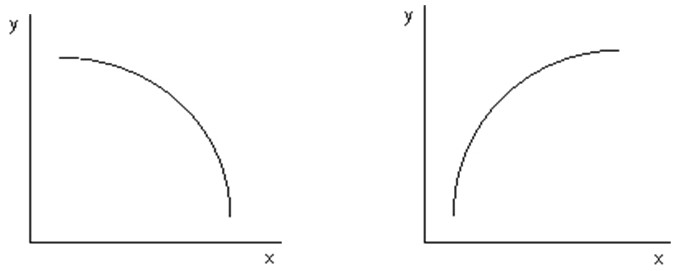
Curvilinear functions are functions that are non-linear in nature. They take many forms such as logarithm functions, log-linear functions, and exponential functions. An exponential function takes the form: F(x) = y = abx where a is not equal to 0 and b is a constant referred to as the base of the exponential function, and b is greater than 0 but not equal to 1. Y is the dependent variable and x is the independent variable and it is the exponent of the constant, b. Therefore, exponential functions are functions that contain a constant base that has a power of a variable exponent. In economics, exponential functions are significant in evaluating the rate of growth or decay of investments or profits. For instance, exponential functions can be used to determine the value of an investment that grows by a constant rate in each period. Other applications of exponential functions are determining the sales of a firm that grow at a constant rate every period, as well as in the models of economic growth or models of epidemics (Heckman & Learner, 2007). The graphs below depict two forms of exponential functions. The graph on the left-hand side shows that as the value of x increases by one unit, the value of decreases by more than one unit. On the other hand, the graph on the right-hand side shows that as the value of x increases by one unit, the value of y increases by more than one unit.
Application of exponential functions to investment
Compound interest – The time value of money
Every economic agent, be it households, firms, or the government, undertakes financial decision-making. Such a process is crucial in that it necessitates the assessment of whether or not expenditures are justified by the benefits they are anticipated to provide. One of the most important financial decisions that economic agents make is a financial investment. Investment decisions entail obtaining an asset and expecting the asset to be worth much more in the future. However, in making such an investment, it is important to note that the cash outflows incurred and the cash inflows earned take place at different periods of time. As a result, it is important to make a comparison of the flow of money that occurs at different times.
Investment incomes are of different forms including: “business earnings, revenues from a toll road, rent from property, interest on a bond, and dividends or capital gains from stock”. In making an investment decision that involves the acquisition of a productive asset, the investor should distinguish between the expenditure (outflow) and receipt (inflow). Cash outflow refers to “the amount of money spent on an investment in the present due to the expectation of the receipt of money in the future” . On the other hand, cash inflow refers to the amount of money received in future periods. A positive return on investment occurs when the anticipated cash inflow is greater than the current outflow. A positive return thus supports the investment decision and therefore the investor should continue with the investment. However, a major problem arises in the comparison of cash outflows and inflows. This problem occurs mainly because cash outflows and inflows take place at different periods of time hence such values are different in that a value received today is not equivalent to a value received tomorrow. Therefore, comparing such values is not logical. In order to facilitate the comparison of different values of investment, it is important to change the values into units of standardized value. This means transforming them into one period of time and then comparing them. The investor should proceed with the investment if the expected benefits outweigh the expenditures .
The problem of comparing values of different periods arises due to the element of interest rate. If the investment is done at a certain rate of interest, the money received in the future will grow according to the interest rate. The interest received in the future is thus the time value of money because the money will grow larger with the passage of time. Different values of different periods of time can be transformed into one period of time either through compounding or discounting. Compounding entails transforming the present values of money into their corresponding future values. This process is mainly used to establish the values of money at the end of a specified investment period. On the other hand, discounting refers to the transformation of future values of money to their corresponding present values. This process is mainly used to determine the initial value of the investment. “Of the two standardization procedures, discounting is the more common in financial decision making,”.
Future values and compounding (single payments)
Compounding is the process of converting present values to future values. This is done in several steps. The first step is to identify the present value of the investment, that is, the initial amount spent on the investment. At the end of the first period of investment, the investment will have grown. The amount will now consist of the initial amount (present value) and the interest earned on the present value (rPV).
FV1 = PV + rPV
FV1 = PV (1+r)
At the end of the second period of investment, the amount of money will have grown and will consist of the money at the end of the first period (FV1) and the interest earned during the second period.
FV2 = FV1 + r FV1
FV2 = FV1 (1+r)
FV2 = PV (1+r) (1+r)
FV2 = PV (1+r)2
This process can continue in order to find the future values of all future periods. This will give “a subscript for the applicable future period which is similar to the numerical value as the exponent for the expression (1+r)”. It is, therefore, possible to obtain a common expression for future values of investment:
FVn = PV (1+r)n
which can also be simplified as: y = abn where a represents the present value (PV), b represents (1 + r) and n is the number of periods of investment. The expression (1+r)n is referred to as the future value interest factor.
Present Values and discounting (single payments)
Discounting is the opposite of compounding and entails transforming the expected future values to present values. To do this, the following procedure is followed:
FVn = PV (1+r)n


PV = FV (PVIF n,r)
In this expression the present value is determined by the value of r, the interest rate, and n, the time period. “The expression, in square brackets, is referred to as the present value interest factor for a single payment, PVIF r,n where r is the interest rate and n is the number of periods” . It is important to realize that the present value of a future value decreases as the discount rate increases and decreases the further into the future the cash flow occurs.
Functions of Two Variables
In the functions discussed above, the dependent variable has been expressed as a function of only one independent variable. However, most functions in economics are functions of two or more independent variables. A good example of a function of two variables is production function. A production function shows the maximum level of output that can be produced with given amounts of inputs (Schmidt & Traub, 2005, p. 288). An example of a production function is the Cobb-Douglas production function which is expressed in general form as: Q = f (L, K) and in specific form as:
Q = ALaKb
where:
- A is the total factor productivity
- L is the quantity of labor inputs used in the production
- K is the amount of capital used in the production
- a is the elasticity of output with respect to labor
- b is the elasticity of output with respect to capital
Although there are many inputs that are used in the production process, the above production function assumes that only capital and labor are used as the factor inputs. A Cobb-Douglas production function is a production function in which the factor inputs are used together. Such inputs can therefore not be substituted for each other. This is different from a linear production function in which the two inputs can be substituted for each other. The Cobb-Douglas production function has special properties:
- Constant returns to scale:
Constant returns to scale implies that if we increase capital and labor by a certain proportion, N, the level of output will also increase by the proportion N.
F(NK, NL, A) = N. F (K, L, A) for all N > 0
This property is also referred to as homogeneity of degree one in K and L. It is important to note that the definition of scale includes only the two rival inputs, capital and labor but does not include the A.
- Positive and diminishing returns to private inputs:
For all K > 0 and L > 0, F (.) exhibits positive and diminishing marginal products with respect to each input.
dF/dk > 0, d2F/dK2 < 0 dF/dL > 0, d2F/dL2 < 0
Therefore, the Cobb-Douglas production function assumes that, holding constant the levels of technology and labor, each additional unit of capital results in positive additions to output, but these additions decrease as more and more capital is added. Similarly, each addition of labor results in positive additions to output, but these additions decrease as more and more labor is added.
- Inada conditions:
The third defining characteristic of the neoclassical production function is that the marginal product of capital (or labor) approaches infinity as capital (or labor) goes to 0 and approaches 0 as capital (or labor) goes to infinity. These properties are called Inada conditions (Barrow & Salai-i-Martin, 2004).
- Essentiality:
An input is essential if a strictly positive amount is needed to produce a positive amount of output. That is, F (0, L) = F (K, 0) = 0.
The specification of a production function enables firms in decision making. Such decisions include: whether or not to use certain inputs and whether to use more of an input and less of the other input. Firms are aided to make such decisions by comparing the marginal productivities of the factor inputs and the prices of the factor inputs. For a linear production function, the equilibrium condition is obtained by dividing the marginal products of the factor inputs with their prices. The ratio gives the marginal product for a shilling spent on each input. For instance, if the ratio of marginal product of labor and the price of labor is greater than the ratio of marginal product of capital and the price of capital, then a firm with a linear production function should use labor and no capital in its production process and vice versa. In a non-linear production function such as the Cobb-Douglas production function, the decisions regarding the utilization of factor inputs are arrived at using the Lagrangian method of constrained optimization which involves maximizing output subject to a cost constraint function or minimization of the firm’s cost subject to output.
In sum, mathematics is an important tool for different types of economic agents. It enables consumers to make decisions about the demand for certain commodities given their prices and the consumers’ incomes. It enables suppliers to make decisions about what to supply and the amounts of supplies to bring to the market. It helps investors to make the right decisions about their investments. Last but not least, it enables firms, through their managers, to make important decisions about the level of production of commodities and services, given the amount of inputs and their prices.
Reference List
Barrow, R., & Salai-i-Martin, X. (2004). Economic Growth. London: MIT Press.
Heckman, J. J., & Learner, E. (2007). Handbook of econometrics, volume 6. London: Elsevier.
Maurice, S., & Thomas, C. (2008). Managerial economics w/ CD (9th ed.). New York, NY: McGraw-Hill.
Schmidt, U., & Traub, S. (2005). Advances in public economics: utility, choice and welfare: a festschrift for Christian Seidl. London: Springer.