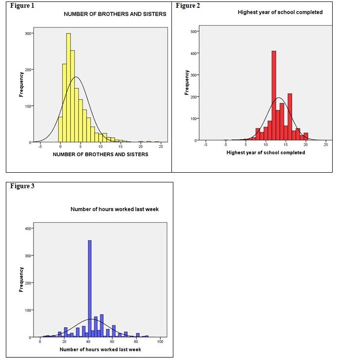
For the three variables in question, the computed means are 42.5 hours worked per week, 13.2 years of educational attainment, and 3.85 siblings. Nominally, the mean for the first independent variable means that Americans typically work either 40 hours (5 days) or an additional half-day on Saturdays. The fact that the mode and median are both at 40 hours alerts us to the reality (see also Figure 3 overleaf) that a five-day workweek is a norm. That the mean is slightly higher than the mode or median shows that a small number of workers do put in extra time.
Table 1: Comparing Measures of Central Tendency
On the matter of educational attainment, a mean and median suggesting that one year of college is representative of the working population are preferable to the mode of 12 years. Barring exceptional circumstances, children do have to stay in school at least until Grade 12. But the truth is that educational attainment is a bimodal distribution because a good number of the youth do go on to take some college and even obtain a degree. And this finding is more important than sadly conceding that families can typically afford to send children only up to Junior College.
The matter of family size is tricky. More often than not, adults of today have two siblings which equates to a family size of three. However, the median reveals that half the sample have more than 3 siblings; the mean of 3.85 siblings reveals the upward pull of a distribution skewed by a substantial number of families with unusually large numbers of children (figure 1 below). A last point in this respect is that sibling count needs to be analyzed by age cohort since the trend toward smaller family sizes makes it likely that the youth have fewer siblings than the middle-aged among us. As well, there are also likely to be significant differences by race.
Job satisfaction is an ordinal variable; the hypothesized independent variables “education” and “age” are scale variables while “rincome” is ordinal. This permits the use of the Pearson correlation coefficient.
Table 2. Correlations Between Job Satisfaction and Independent Variables: Total Sample
On the whole, the mean rating for job satisfaction is 1.68 or close to “moderately satisfied” (on a four-point scale where 1= “very satisfied” and 2 = “moderately satisfied”). Given a standard deviation of 0.77, two-thirds of the sample would theoretically lie between a job satisfaction rating of 0.91 (non-existent) and 2.45, still in the “moderately satisfied” portion of the scale.
SPSS flagged solely the inverse correlation between age and job satisfaction as being significant at the 0.99 confidence level. This means only one chance in a hundred that the relationship between the two variables could be due to chance. In real-world terms, a correlation of -0.089 is hardly meaningful. Accepting it at face value, the finding suggests that older workers are more likely to be satisfied with their work. This is usually accounted for by greater skill or going up the career ladder. Since this happens to only a minority of workers, the relationship is not especially remarkable.
The findings remain even when switching to Spearman’s rho to account for the ordinal nature of the dependent variable:
Table 3. Spearman’s Rank-Order Correlations
For the most part, the relationship among satisfaction, education, and income does not differ materially for men and women. Table 4 (appended) shows that partial correlations controlled for sex do not meet the required significance level of even 0.05 except in the case of the relationship between job satisfaction and income. This stands to reason since earning more money permits one many more comforts and amenities and thus increased job satisfaction.
Table 4. Partial Correlations, Controlling for Gender